High-speed golf swings represent nonlinear biomechanical systems in which passive dynamics (drift) increasingly dominate over active torques (control) as angular velocities rise. We formalize this phenomenon using the Drift-Control Ratio (DCR),
Within the simplified planar model used here, example calculations suggest that DCR can increase by more than two orders of magnitude from the top of the backswing to impact. This is a statement about the relative magnitudes of two modeled acceleration sets in a declared projection. DCR alone does not determine finite-horizon reachability, path-correction authority, or an impact outcome.
We distinguish the drift-affected instantaneous velocity set, the input-only control-effect set, and the finite-horizon reachable set. A constant-additive-drift counterexample shows why large scalar DCR can translate a reachable set without shrinking it. The former control-cone, pancake, and drift-tube descriptions are retained only as unvalidated hypotheses whose evaluation requires a horizon, admissible controls, task metric, uncertainty model, and event-level outcome.
Technical claim (Bounded): Within a declared model, DCR compares the magnitudes of modeled drift acceleration and the largest modeled input acceleration in chosen coordinates. DCR alone does not prove or determine finite-horizon reachability, path-correction authority, an impact outcome, or a locked-in golfer state.
Population: Declared dynamical models and admissible input sets; no golfer population is inferred.
Valid conditions:
Drift and input accelerations are evaluated at the same state in the same coordinates.
The admissible input set, weighting, norm, and regularization are declared.
Uncertainty (Unquantified): Model-form, input-set, coordinate, norm, parameter, and measurement uncertainty are not quantified by the scalar ratio.
Limitations:
DCR depends on the declared state, input set, projection, weighting, norm, and regularization.
The analytical counterexample is not a participant-level golf validation or a coaching prescription.
Falsifier:
The declared constant-additive-drift system changes reachable-interval width when only constant drift changes.
A scalar DCR value alone uniquely determines a finite-horizon reachable set across admissible systems.
Data provenance: No participant dataset is used; the governing evidence is an exact analytical constant-drift counterexample and its executable regression test.
Next validation gate: Run preregistered finite-horizon, three-dimensional golfer-club perturbation studies with declared controls, uncertainty, and impact outcomes.
This article asks a narrow modeling question: how large is passive acceleration relative to the acceleration available from a declared input set? That ratio does not, by itself, say whether a golfer can correct a path or outcome.
The Drift-Control Ratio (One Magnitude Comparison)
DCR compares modeled drift acceleration with the largest modeled input acceleration in the same chosen coordinates. It is not a muscle-power measurement, and a large value is not a certificate that control has disappeared.
Think of a uniform river current: A stronger current moves every possible canoe endpoint downstream, but it does not automatically reduce the range of endpoints the paddles can add around that downstream motion. Whether the endpoint range actually narrows depends on how the current, boat, paddle limits, and route change over time.
Three Different Questions
The possible velocity right now, the change attributable to the available input right now, and the states reachable by impact are different mathematical objects. DCR summarizes neither their shape nor their future evolution.
Practical consequence: A late correction may be small in a particular model, but that conclusion must come from a bounded trajectory calculation tied to the impact task—not from the scalar ratio alone.
Path and Face Hypotheses
The idea that path corrections become narrow while face corrections remain wide is a testable hypothesis. It has not been established here with a three-dimensional golfer-club model or measured admissible controls.
What the test needs: Declare the time remaining to impact, allowable inputs, coordinates and task metric, parameter uncertainty, and the impact quantity being corrected.
Key Takeaway: A large DCR flags a modeled magnitude imbalance worth investigating. It does not prescribe technique or prove that a future correction is unavailable.
Review the governed technical claim and its limits.
Every theory faces scrutiny. Here's what skeptics and alternative perspectives say:
Motor Control Theory:
Is "Loss of Control" Actually "Gain of Precision"?
Critics citing the **Signal-Dependent Noise** theory (Wolpert et al.) argue that high torque generation introduces proportional motor noise. Therefore, the high DCR observed in the late downswing (where active torque is minimal relative to drift) may be a functional adaptation to *minimize* noise, not a loss of agency. By "riding the drift," the golfer avoids the inaccuracy inherent in high-force corrections.
Our Response: DCR does not measure trajectory controllability or signal-to-noise ratio. Those require a controller, an admissible input set, a noise model, a horizon, and a task-level correction target. The noise-minimization interpretation and the loss-of-agency interpretation are both hypotheses until tested under the same declared model and data.
Dimensionality Critique:
The "Steering Wheel" Fallacy (Axial Decoupling)
The DCR analysis focuses on the high inertia of the swing plane. Skeptics argue that accuracy depends primarily on the **Clubface Angle** (axial rotation), which has very low inertia ($I_{axial} \ll I_{plane}$). Since the golfer retains high authority over axial rotation throughout the downswing, the "loss of path control" is irrelevant to the outcome.
Our Response: Planar DCR does not determine arrival-time reachability or face-angle variance. Testing that coupling requires a spatial model, bounded path and axial inputs, event-time sensitivity, and an impact metric. The present planar ratio cannot adjudicate the critique.
Impedance Control:
Stiffness vs. Torque
The affine model $\dot{x} = f(x) + G(x)u$ treats control purely as torque ($u$). Critics argue that skilled golfers modulate **Mechanical Impedance** (stiffness/damping) to reject disturbances without active feedback. By stiffening the wrists ("Effective Plant"), the golfer can maintain control even when DCR suggests torque authority is lost.
Our Response: Changing stiffness or damping changes the effective plant, its drift field, and potentially its admissible input set. A DCR value is therefore conditional on the declared impedance model. Subject-specific perturbation, kinematic, kinetic, and activation measurements would be needed to identify that plant in golfers.
Note: Scientific discourse thrives on debate.
These critiques strengthen our understanding by defining the boundaries of the model.
2 Introduction
Golf swings can involve large clubhead and segment velocities. Sensorimotor and electromechanical delays constrain some feedback pathways, but they do not establish that every within-downswing adjustment is impossible.
This mirrors a common theme in high-speed movement: the system transitions from control-dominated to drift-dominated dynamics as velocity increases.
Building on the foundational framework established in Affine Control Interpretation of the Golf Swing, we analyze the relative magnitude of declared drift and bounded input acceleration in \(\dot{x} = f(x) + G(x)u\). The decomposition is model-based bookkeeping; it does not identify physiological cause or quantify controllability by itself.
Our goal is to provide a model-bounded treatment of this phenomenon through:
Multibody dynamic derivations of drift and control.
Accessibility and Gramian boundaries for interpreting the scalar ratio.
Reachable-set distinctions and an executable counterexample to scalar-DCR overreach.
Validation requirements for path, event-time, and clubface-outcome hypotheses.
This approach treats the Drift-Control Ratio as a useful diagnostic for the model’s drift-versus-input balance. Its empirical value depends on calibration against measured swing data.
3 System Modeling: The 3-Link Arm–Forearm–Club Model
We model the golfer–club chain as a 3-DOF planar system:
A naïve application of the Euclidean norm to the full state vector drift \(\|f(x)\|\) mixes units of velocity (\(\text{rad/s}\)) and acceleration (\(\text{rad/s}^2\)). To ensure physical meaningfulness, we restrict our definition to the dynamic fiber of the tangent bundle (the acceleration subspace), comparing the generalized forces (or equivalent accelerations) of drift against the available control authority.
The quadratic scaling of drift versus linear scaling of control is the core mechanism behind DCR blow-up.
The full state-space norm \(\|f(x)\|\) is dimensionally heterogeneous, so this scaling argument applies only to the acceleration block \(a_{\text{drift}}(x)\).
This scaling disparity is the kinetic manifestation of the Force Taxonomy established in Part 3 of the framework. The drift term \(f(x)\) aggregates the configuration-dependent potential forces (\(\tau_{\text{config}}\)) and the velocity-dependent Coriolis/centripetal forces (\(\tau_{\text{vel.\,drift}}\)). While the former are bounded, the latter scale quadratically with swing speed. Consequently, the “Inertial Memory” of the system (embedded in \(f(x)\)) can become large relative to the “Current Agency” available through \(G(x)u\). In this model, that scaling supports the early-delivery interpretation used by the ZTCF family baseline, but it does not by itself prove a universal coaching rule.
NoteScope Limitation: Planar vs. Axial Dynamics
This planar model (\(q \in \mathbb{R}^3\)) captures transport mechanics (path velocity) but excludes axial shaft rotation (supination/pronation). As discussed in Section 6.1, planar DCR is only a path-projected magnitude ratio. It does not establish path controllability, and it provides no certificate for face controllability in the omitted spatial subsystem.
4 Drift-Control Ratio (DCR)
We define the Drift-Control Ratio (DCR) as the ratio of modeled drift to bounded modeled control capacity in the same declared acceleration or task-projected space.
ImportantDimensional Consistency Note
A naïve application of the Euclidean norm to the full state vector drift \(\|f(x)\|\) mixes units of velocity (\(\text{rad/s}\)) and acceleration (\(\text{rad/s}^2\)). To ensure physical meaningfulness, we restrict our definition to the dynamic fiber of the tangent bundle (the acceleration subspace), comparing the generalized forces (or equivalent accelerations) of drift against the available control authority.
ImportantCanonical DCR Definition (Site-Wide)
Across this website the canonical Drift-Control Ratio is \[
\boxed{\;\mathrm{DCR}_{W,\mathcal U}(x) \;:=\;
\frac{\|W a_{\mathrm{drift}}(x)\|}
{\sup_{u\in\mathcal U(x)}\|W B_a(x)u\|+\varepsilon}\;}
\] where \(a_{\mathrm{drift}}\) and \(B_a u\) are expressed in the same acceleration space, \(W\) selects and weights the reported coordinates or task directions, \(\mathcal U(x)\) is the admissible control set, and \(\varepsilon\) is a declared regularizer. A mass-weighted norm, Euclidean norm, or task projection is permitted only when reported explicitly. The denominator is available capacity, not the instantaneous policy realization. DCR is therefore conditional on the state, effective plant, projection, norm, and capacity model. The normative definition is maintained in the Mathematical Notation Reference.
This policy-dependent drift-to-realized-input ratio (DIR) describes what a controller actually did. It is not DCR and does not measure remaining capacity.
Using approximations where drift forces scale quadratically with velocity (\(C\dot{q} \sim \dot{q}^2\)):
If available torque decreases during peak velocity because of force-velocity constraints, the denominator shrinks while the numerator grows. The timing and magnitude of that effect should be checked against subject-specific data.
Estimated result (planar model):\[
\mathrm{DIR}_{W}(t) \text{ increases by approximately } 100\times-300\times \text{ across the downswing.}
\](This policy-dependent estimate is derived from the planar model above with typical parameter values; it is not a DCR capacity estimate, and empirical validation against instrumented swing data is needed.)
4.1 Dimensional Analysis and Norm Dependence
Now, a careful reader will wonder: does this ratio depend on how we measure things? Of course it does—and that’s worth thinking about carefully, because the answer reveals what’s really going on.
4.1.1 The Norm Problem (Stated Clearly)
The Euclidean 2-norm is our default choice: \[
\|f_{acc}\|_2 = \sqrt{\sum_i (f_{acc})_i^2}.
\]
But alternative norms yield numerically different DCR values: - Infinity norm (max absolute value): \(\|f_{acc}\|_\infty = \max_i |f_{acc}|_i\) - Weighted norm (inertia-scaled): \(\|f_{acc}\|_M = \sqrt{f_{acc}^\top M f_{acc}}\) - Task-space norm: norms defined in operational space (e.g., clubhead acceleration)
A system with DCR\(_2 = 47.3\) might have DCR\(_\infty = 89.2\) or DCR\(_M = 12.1\). The absolute numbers depend on the measuring stick.
4.1.2 An Inertia-Weighted Option
For golf biomechanics, we recommend the inertia-weighted norm: \[
\|f_{acc}\|_M = \sqrt{f_{acc}^\top M(q) f_{acc}}.
\]
Because \(M(q)\) is the mass matrix, this weighting incorporates configuration-dependent inertia. It does not turn acceleration into kinetic energy, and it is not uniquely preferred for every task. A task-space metric may be more appropriate when the declared outcome is clubhead path or an impact variable.
4.1.3 Statement and Recommendation
The physically meaningful conclusion is therefore:
“In the planar examples considered here, the ratio of drift-generated acceleration to control-available acceleration increases strongly from the top of the backswing to impact. The qualitative pattern is robust in these examples, but exact monotonicity and numerical thresholds remain norm- and model-dependent.”
For practice: 1. Always report the norm used in DCR calculations. 2. Report growth ratio (e.g., “100× increase from top to impact”) rather than absolute threshold values. 3. Justify the metric for the task rather than treating any one norm as universal.
WarningCross-Joint Comparison Caveat
DCR values for different degrees of freedom (e.g., shoulder rotation vs. wrist flexion) are not directly comparable without normalization. Rotational DOFs (rad/s²) and translational DOFs (m/s²) have different physical units; even within the rotational subspace, joints with different inertias will exhibit different DCR magnitudes for identical mechanical situations. The inertia-weighted norm \(\|f_{acc}\|_M\) partially addresses this by weighting by \(M(q)\), but comparisons across subsystems should still be interpreted cautiously. DCR is most reliable as a within-DOF, temporal measure (tracking how a single DOF’s drift-control ratio evolves over the swing) rather than as a cross-DOF comparison.
Both the reported number and its interpretation remain conditional on the declared measuring stick and model.
5 DCR and Reachability: What the Scalar Does Not Prove
For \(\dot{x}=f(x)+G(x)u\) with admissible control set \(\mathcal{U}(x)\), three objects must remain separate:
The drift-affected instantaneous velocity set\(f(x) + G(x)\mathcal{U}(x)\).
The input-only control-effect set\(G(x)\mathcal{U}(x)\).
The drift translates the first set relative to the origin. It does not change the shape of the second set at the same state. Over a finite horizon, state dependence in \(f\), \(G\), and \(\mathcal{U}\) can translate, rotate, stretch, or contract the reachable set. A scalar norm ratio does not encode those effects. DCR alone does not determine finite-horizon reachability.
The Hamiltonian support function makes the same distinction:
The first term shifts support in direction \(p\); the second supplies directional control support. Their norm ratio cannot recover the support function or its evolution to an impact event.
5.1 Executable Constant-Drift Counterexample
Consider \(\dot{x}=d+u\) with \(|u(t)|\leq\bar{u}\). For constant \(d\),
Its center is \(x_0+dT\), while its width is \(2\bar{u}T\), independent of \(d\). With \(x_0=0\), \(\bar{u}=1\), and \(T=1\), zero drift gives \([-1,1]\) and \(d=100\) gives \([99,101]\). The DCR-like magnitude ratio changes from \(0\) to \(100\), but the reachable width remains \(2\). The checked implementation is src/affine_control/reachability.py::constant_additive_drift_interval, exercised by tests/test_dcr_reachability_contract.py.
This counterexample does not claim that golf-swing drift is constant. It proves the narrower logical point: drift magnitude alone cannot establish reachable-set shrinkage.
5.2 What a DCR Threshold Means
If a declared DCR equals 10, the reported drift norm is ten times the largest input-effect norm in that projection and metric. Nothing discontinuous happens at 10. It is not a controllability, accessibility, saturation, or reachable-set threshold.
Claims about whether path correction becomes too small for a specified task remain unavailable until a governed trajectory study declares the horizon, state-dependent admissible control set, state coordinates, task metric, model and measurement uncertainty, and impact-event outcome with its acceptable tolerance.
DCR also does not predict separation between an observed trajectory and a Zero Torque Counterfactual (ZTCF). That separation must be obtained from the declared forward interventions, with divergent states and model assumptions reported.
6 The Control-Cone Analogy as an Unvalidated Hypothesis
For fixed \(x\), the short-time limit \(\mathcal{R}(\Delta t;x)\to\{x\}\) is a singleton, not a direction cone. A first-order rescaling instead gives the drift-affected velocity set:
under the usual local regularity assumptions. Subtracting the nominal drift contribution leaves the control-effect set \(G(x)\mathcal{U}(x)\). Neither set is generally a cone; bounded controls more often produce a translated compact set.
The earlier control-cone, drift-tube, and pancake pictures can therefore serve only as names for possible finite-horizon anisotropy. They are unvalidated hypotheses, not consequences of high DCR or analogues of relativistic causal structure. A governed computation might support a narrow task-projected reachable corridor in a particular model, but it must report the horizon, admissible controls, task metric, uncertainty, and impact-event outcome.
6.1 Accessibility and Gramian Boundaries
Lie-bracket rank conditions concern local accessibility under their stated regularity assumptions. They do not show that multiplying the drift magnitude reduces accessibility rank, nor do they turn a norm ratio into a finite-horizon controllability certificate.
For a trajectory-linearized perturbation model
\[
\delta\dot{x}=A(t)\delta x+B(t)\delta u,
\]
a controllability Gramian depends on \(A(t)\), \(B(t)\), the time horizon, and the input metric. There is no general law making its planar eigenvalues or ellipsoid aspect ratio a scalar function of DCR. Establishing a pancake-shaped nonlinear reachable set would require an explicit spatial model, converged reachability computation, admissible controls, and uncertainty treatment.
6.2 Event-Level Path and Face Tests
Different path and axial inertias can motivate a hypothesis that late path authority and face authority differ. DCR does not validate that hypothesis. A suitable study would apply the same declared bounded controls to a spatial model through an impact event, then report directional changes in path, arrival time, and face angle in the impact-event outcome. It would also test sensitivity to inertial parameters, shaft dynamics, impedance assumptions, and uncertainty. Neither planar DCR nor a quoted closure rate supplies those missing results.
7 Bounded DCR Validation Protocol
This protocol asks a narrower question than whether DCR is an appealing description: does a declared DCR add held-out information about a declared correction task beyond the state already known to the analysis? The analytic counterexamples come first. A positive association or prediction result cannot override a counterexample to a universal or theorem-level claim.
ImportantAuthority Boundary
The current executable cases are analytic or deterministic synthetic systems. Parameter bounds are assumed inputs to those systems. No participant or golfer data are measured or estimated, and golfer task outcomes remain unavailable. This exploratory output is not coaching, clinical, design, causal, or population authority.
7.1 Protocol Declaration
Every run fails closed unless it records all of the following fields before results are examined:
Required Field
Declaration
State and coordinates
Named initial-state values, coordinate frame or chart, and units.
Input set and bounds
Named admissible inputs, lower and upper bounds, units, and whether bounds vary with state.
Scaling and norm
Coordinate scaling or weighting and the exact norm used for DCR and task projections.
Finite horizon
Start state or phase, terminal time or stopping rule, and units.
Event definition
Guard surface, crossing direction, reset/contact rule, and event-time convention.
Task metric
Quantity being corrected, tolerance, and whether error is evaluated at fixed time or at the event.
Uncertainty model
Declared parameter/model set or probability model; unavailable uncertainty is reported as unavailable.
Solver and tolerance
Engine, solver and revision, step or analytic method, convergence test, and numerical tolerance.
The executable ReachabilityProtocol binds those declarations. The scalar and planar system regressions extend src/affine_control/reachability.py; the zero-gradient and rank-deficient cases call the protected #4013 constant_additive_drift_interval API rather than defining a competing reachability calculation. Protocol and hypothesis records live in the separate orchestration layer src/affine_control/reachability_protocol.py.
7.2 Analytic and Deterministic Regression Matrix
The regression suite fixes six systems before any positive interpretation:
System
Frozen Regression
What It Can and Cannot Establish
constant additive drift
With \(x_0=0\), \(\bar u=1\), and \(T=1\), drift 0 and 100 give \([-1,1]\) and \([99,101]\); both widths are 2.
Drift can translate a reachable set without shrinking it. This refutes universal scalar sufficiency, not a golf-specific effect.
state-dependent drift
\(\dot x=1+u\) and \(\dot x=x+u\), both at \(x_0=1\) with instantaneous DCR 1, have widths 2 and \(2(e-1)\approx3.4366\).
Equal instantaneous DCR does not fix finite-horizon width.
rank-deficient input map
For \(G=[1,0]^\mathsf{T}\), drift \((0,10)\), \(\bar u=1\), and \(T=1\), the box is \([-1,1]\times\{10\}\), input-map rank is 1, and area is 0.
A norm ratio does not encode directional rank or controllability.
saturation
A requested scalar correction of 2 with gain 1 and input bound 0.5 applies 0.5 and preserves an unmet residual of 1.5.
Constrained optimal correction depends on the task request and bounds, not DCR alone.
contact and event timing
Two height-1 cases with velocities \(-1\) and \(-3\), drift acceleration \(-9\), and control acceleration \(+1\) reach the event at about 0.3904 and 0.25. Event-velocity sensitivities to control acceleration are about 0.2425 and 0.2.
The same drift/control magnitude comparison can accompany different event maps because baseline state and speed differ.
model and parameter perturbations
For \(\dot x=ax+u\), \(x_0=1\), \(\bar u=1\), \(T=1\), and \(a\in\{0.8,1.0,1.2\}\), center spans \([2.2255,3.3201]\) and width spans \([3.0639,3.8669]\).
Assumed parameter variation is published as an envelope rather than hidden behind one ratio.
All values above are analytic or modeled quantities from declared synthetic systems. They are not measurements. The exact numeric checks are in tests/test_dcr_event_sensitivity_protocol.py; a failed event, invalid bound, missing field, or nonfinite value is an explicit failure state rather than a substituted result.
7.3 Predeclared Hypotheses and Promotion Gates
Association hypothesis: Test whether DCR remains associated with the declared task error after adjustment for baseline state, speed, and control authority. Report the coefficient, uncertainty interval, dependence structure, and missingness rule. Association does not imply intervention effect.
Prediction hypothesis: Test whether adding DCR to that baseline reduces held-out task-error RMSE by at least a predeclared margin. Use group- or participant-held-out folds for participant data; the deterministic fixture uses leave-one-out cross-validation only to regression-test the calculation.
Theorem-level hypothesis: Test any claim that scalar DCR alone determines correction authority against the complete counterexample matrix. One valid counterexample rejects the universal claim even if association or prediction is positive in a narrower dataset.
The current baseline-exact synthetic fixture gives both baseline and DCR-augmented held-out RMSE below the declared \(10^{-10}\) tolerance. Its incremental-prediction outcome is therefore null, not positive. The theorem-level scalar-sufficiency hypothesis is negative because the analytic counterexamples refute it. Association in golfers is unavailable because no participant data enter this protocol. Null and negative results remain in the ledger alongside supported and unavailable results; they are not filtered from publication.
For future measured data, preprocessing, folds, thresholds, model revisions, and hypothesis tiers must be frozen before inspecting outcomes. Cross-validation must compare the baseline state, speed, and control authority model with the same model plus DCR. Uncertainty must cover held-out error and declared parameter/model perturbations. A result can be promoted only within that dataset, model, event, task metric, and uncertainty envelope.
8 Stability and Clubface Variance: Required Model
Let clubface angle be \(\phi=h(q)\). A local event-variance analysis may start from
\[
\delta\dot{x}=A(t)\delta x+B(t)\delta u,
\qquad
\delta\phi=H(t)\delta x,
\]
but it must also declare the feedback policy, disturbances, measurement noise, initial covariance, state-transition model, and impact-event sensitivity. DCR contains none of these objects. In particular, a large norm ratio does not imply a large state Jacobian or exponential error growth. The previous claim that path drift enforces face error is therefore withdrawn; that relationship is unavailable pending an event-level uncertainty study.
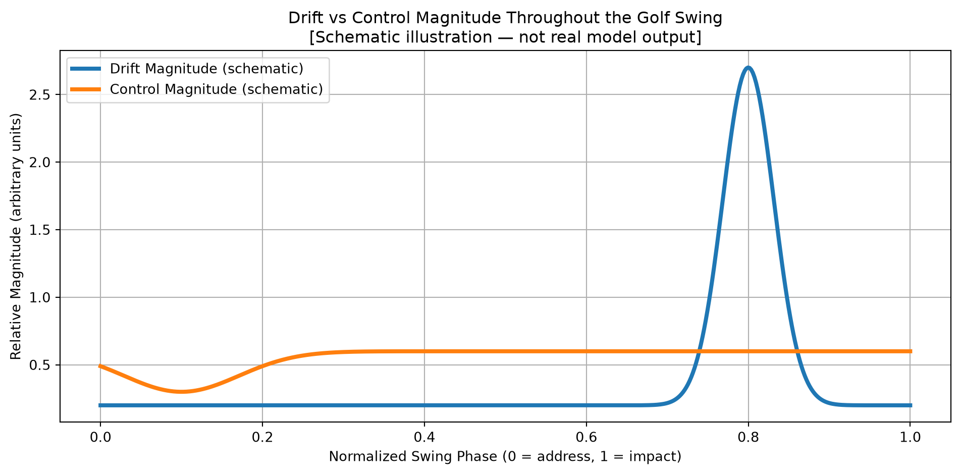
9 Schematic Illustration: Drift vs Control Magnitude
NoteSchematic Only — Not Real Data
The plot below is a schematic illustration generated from qualitatively motivated mathematical functions. It is not output from a real biomechanical model or motion-capture measurement. The functional forms (exponential growth of drift near impact, gradual decay of control authority) are chosen to reflect the qualitative pattern described in the theoretical analysis. Calibrated curves from an instrumented swing model would be needed to validate the specific magnitudes and timing.
Code
import numpy as npimport matplotlib.pyplot as pltt = np.linspace(0, 1, 500)drift =0.2+2.5* np.exp(-((t -0.80)**2) /0.002)control =0.6-0.3* np.exp(-((t -0.10)**2) /0.01)plt.figure(figsize=(10, 5))plt.plot(t, drift, label="Drift Magnitude (schematic)", linewidth=3)plt.plot(t, control, label="Control Magnitude (schematic)", linewidth=3)plt.title("Drift vs Control Magnitude Throughout the Golf Swing\n""[Schematic illustration — not real model output]")plt.xlabel("Normalized Swing Phase (0 = address, 1 = impact)")plt.ylabel("Relative Magnitude (arbitrary units)")plt.legend()plt.grid(True)plt.tight_layout()plt.show()
10 Limitations of This Analysis
WarningLimitations of This Analysis
Planar model only: The 3-DOF model captures path dynamics but excludes axial rotation. A spatial model is required before any directional reachable-set shape can be assessed; the pancake picture remains an unvalidated hypothesis.
Norm and model dependence: DCR values and their time trend depend on the declared projection, norm, input bounds, and model. No scalar DCR threshold establishes reachable-set collapse.
Static torque bounds: We assume fixed physiological torque limits. In reality, torque capacity varies with joint angle and velocity (the force-velocity relationship), which could modify the DCR profile.
No stochastic analysis: This deterministic analysis does not account for motor noise. The interplay between DCR and signal-dependent noise (Wolpert et al.) deserves separate treatment.
Rigid body assumption: Shaft flexibility and soft tissue compliance may modify the effective inertia and hence the DCR, particularly near impact.
No golf-model finite-horizon result: The bounded protocol above contains analytic and deterministic synthetic cases, not a governed reachable set for a calibrated golfer-club model. Path correction, arrival-time adjustment, and impact tolerances in golfers remain unavailable pending the spatial, event-level study described in Section 6.1.
11 Conceptual Linkages
To place this analysis within the broader AffineDrift framework:
Implicit Assumptions:
Drift Invariance: We assume that the passive drift field \(f(x)\) remains structurally independent of the input mechanism, a condition formally proven in Proposition 1 of the core theory.
Torque Bounds: The DCR analysis assumes physiological limits on \(\tau\). Bounded inputs do not by themselves make the modeled system structurally underactuated or establish a ballistic phase.
Cross-References:
The Drifter Manifesto: For the foundational derivation of the affine form \(\dot{x} = f(x) + G(x)u\).
Theory Part 3 (Force Taxonomy): For the detailed breakdown of the drift components (Inertial, Coriolis, Centripetal) that drive the DCR explosion.
Intentional Constraint Collapse: A separate hypothesis about early organization that must not be treated as a reachable-set consequence of DCR.
Zero Torque Counterfactual (ZTCF): A declared input-removal intervention. It is not an infinite-DCR limit and must be reported with its model assumptions.
12 External Resources
NoteCurator’s Note
The following resources are selected to provide authoritative grounding for the concepts of Drift-Control Ratio (DCR), Signal-Dependent Noise, and the Relativistic Analogy.
<div class="youtube-embed">
  <iframe src="https://www.youtube.com/embed/vuZmaSyJpUY"
          title="Phase Portrait for Double Well Potential"
          allow="accelerometer; autoplay; clipboard-write; encrypted-media; gyroscope; picture-in-picture"
          allowfullscreen></iframe>
</div>
<h3>Phase Portrait for Double Well Potential - Steve Brunton</h3>
<div class="resource-description">
  <p>
    <strong>Why it fits:</strong> A masterclass in visualizing nonlinear dynamics. Brunton demonstrates how to construct the "Drift Field" ($f(x)$) for a system with multiple equilibria, directly analogous to visualizing the swing's drift dynamics.
  </p>
  <ul>
    <li><strong>Seek:</strong> 0:00 (Problem Setup), 10:48 (Global Phase Portrait).</li>
    <li><strong>Prereqs:</strong> Basic ODEs, Linearization.</li>
  </ul>
</div>
<a href="https://www.youtube.com/watch?v=vuZmaSyJpUY"
   class="resource-link"
   target="_blank"
   rel="noopener">
  Watch Video →
<span class="sr-only">(opens in a new tab)</span></a>
<h3>Computational Principles of Sensorimotor Control - Daniel Wolpert</h3>
<div class="resource-description">
  <p>
    <strong>Why it fits:</strong> The canonical source for Signal-Dependent Noise. Wolpert explains why "trajectory planning" fails in high-noise regimes and why optimal control (managing the variance) replaces it.
  </p>
  <ul>
    <li><strong>Seek:</strong> 19:37 (Motor Noise is Signal Dependent), 29:04 (The Demise of the Desired Trajectory).</li>
    <li><strong>Prereqs:</strong> Probability, Control Theory basics.</li>
  </ul>
</div>
<a href="https://www.youtube.com/watch?v=ikEzzJLrGWU"
   class="resource-link"
   target="_blank"
   rel="noopener">
  Watch Video →
<span class="sr-only">(opens in a new tab)</span></a>
<div class="youtube-embed">
  <iframe src="https://www.youtube.com/embed/_Az608TI-NI"
          title="The Paradox of Human Performance"
          allow="accelerometer; autoplay; clipboard-write; encrypted-media; gyroscope; picture-in-picture"
          allowfullscreen></iframe>
</div>
<h3>The Paradox of Human Performance - Neville Hogan</h3>
<div class="resource-description">
  <p>
    <strong>Why it fits:</strong> Hogan articulates the fundamental conflict between slow biological hardware and fast performance, introducing Impedance Control as the solution—a key parallel to the "Effective Plant" concept.
  </p>
  <ul>
    <li><strong>Seek:</strong> 0:00 (The Paradox), 15:00 (Impedance as a Dynamic Primitive).</li>
    <li><strong>Prereqs:</strong> Mechanical Impedance concepts.</li>
  </ul>
</div>
<a href="https://www.youtube.com/watch?v=_Az608TI-NI"
   class="resource-link"
   target="_blank"
   rel="noopener">
  Watch Video →
<span class="sr-only">(opens in a new tab)</span></a>
<h3>What is Relativity? - Sean Carroll</h3>
<div class="resource-description">
  <p>
    <strong>Why it fits:</strong> Explains relativistic light cones and clarifies why they should not be used as evidence for mechanical reachable-set geometry. The comparison is pedagogical only; the systems do not share a reachability contract.
  </p>
  <ul>
    <li><strong>Seek:</strong> 20:30 (What are Light Cones?), 28:45 (Implications of Relativity).</li>
    <li><strong>Prereqs:</strong> None (Conceptual).</li>
  </ul>
</div>
<a href="https://www.youtube.com/watch?v=hZsIwDXaN0E"
   class="resource-link"
   target="_blank"
   rel="noopener">
  Watch Video →
<span class="sr-only">(opens in a new tab)</span></a>
13 See Also
For an applied counterfactual modeling study examining how drift and active torque split during proximal-to-distal energy handoffs in the golf downswing, see Proximal-to-Distal Energy Transfer in the Golf Swing.
14 Acknowledgments
Computational modeling assistance and structured drafting support for this article were provided by ChatGPT (OpenAI). All theoretical content, arguments, and conclusions are the work of the named author.
Every theory faces scrutiny. Here's what skeptics and alternative perspectives say:
Is "Loss of Control" Actually "Gain of Precision"?
Critics citing the **Signal-Dependent Noise** theory (Wolpert et al.) argue that high torque generation introduces proportional motor noise. Therefore, the high DCR observed in the late downswing (where active torque is minimal relative to drift) may be a functional adaptation to *minimize* noise, not a loss of agency. By "riding the drift," the golfer avoids the inaccuracy inherent in high-force corrections.
The "Steering Wheel" Fallacy (Axial Decoupling)
The DCR analysis focuses on the high inertia of the swing plane. Skeptics argue that accuracy depends primarily on the **Clubface Angle** (axial rotation), which has very low inertia ($I_{axial} \ll I_{plane}$). Since the golfer retains high authority over axial rotation throughout the downswing, the "loss of path control" is irrelevant to the outcome.
Stiffness vs. Torque
The affine model $\dot{x} = f(x) + G(x)u$ treats control purely as torque ($u$). Critics argue that skilled golfers modulate **Mechanical Impedance** (stiffness/damping) to reject disturbances without active feedback. By stiffening the wrists ("Effective Plant"), the golfer can maintain control even when DCR suggests torque authority is lost.