Superposition in Affine Control Systems via Newton–Euler, Lagrangian, and Screw-Theoretic Formulations
Plain-Language Summary
This article shows that control forces add together cleanly in our swing equations. We test this rule across three standard ways to write the laws of motion.
Key Takeaways
- Input superposition holds strictly for instantaneous generalized forces and accelerations.
- State-space trajectories do not superpose globally because velocity-dependent drift is nonlinear.
- Equivalence is proven across Newton-Euler, Lagrangian, and screw-theoretic formulations.
This article develops a rigorous derivation of superposition with respect to inputs for mechanical systems whose dynamics are affine in control. We work in three parallel formalisms: Newton–Euler equations, Lagrangian mechanics (including Lagrange–d’Alembert), and screw-theoretic / spatial vector mechanics. In each framework we explicitly derive the control-affine structure
\[ \dot x = f(x) + \sum_{i=1}^m g_i(x) u_i, \]
for finite-dimensional mechanical systems actuated by generalized forces, and prove that applied generalized loads depend linearly on the declared load inputs, while acceleration is affine and its increment relative to zero input is linear at fixed state. This yields a precise superposition principle: although trajectories in state space do not superpose in general (due to nonlinearity), the effects of distinct input channels on generalized forces and accelerations do. We provide worked examples in each formulation (a single pendulum, a planar 2R manipulator, and a spatial single-link model) and show how to decompose motion into contributions from gravity, Coriolis/centrifugal effects, and individual actuators.
In the AffineDrift framework, a Zero Torque Counterfactual (ZTCF) family requires a well-posed model and a declared zero-input intervention. Such a baseline can also be defined in nonaffine systems; affinity supplies the additional exact identity for input increments. Setting the modeled torque to zero leaves the function \(f\) unchanged, but a forward counterfactual evaluates it along a different evolving state. The split is conditional on the state, inputs, and contact assumptions and does not identify intention or physiological effort.
At a specified state in a torque-driven model, applied load increments produce acceleration increments that add. The zero-input acceleration must be included once, not once for each input. A snapshot calculation concerns acceleration; delivered clubhead speed also depends on the preceding trajectory.
The same posture and velocity must be used for every term. In a two-hand grip, changing applied torque also changes the constraint reactions. Those reactions must be solved consistently. Muscle force cannot generally be recovered uniquely from the total joint torque, and an additive equation does not make its physical causes independent.
Earlier muscle work, ground impulse, geometry, and elastic storage affect the arriving state. A forward counterfactual then follows its own state and contact events. This is how the snapshot calculation connects to the whole swing without treating several different swing trajectories as additive.
1 Introduction
At fixed state, define \(\mathcal F_x(u)=f(x)+G(x)u\). The exact identity is \[ \mathcal F_x(u_1+u_2)=\mathcal F_x(u_1)+\mathcal F_x(u_2)-\mathcal F_x(0). \] The total map is affine; \(\mathcal F_x(u)-\mathcal F_x(0)\) is linear. Every term uses the same complete state, parameters, and contact mode. These are model-conditioned contributions to the instantaneous state derivative, not independently identified shares of a finite swing outcome.
Superposition is often invoked informally in robotics and biomechanics: one speaks of “the gravitational torque,” “the Coriolis torque,” “the control torque,” as if these were independently meaningful and add linearly to produce the net motion. At the same time, the underlying dynamics are nonlinear in configuration and velocity, so naïve trajectory superposition is false. This tension is a constant source of conceptual confusion.
The correct statement is more modest but powerful:
For a mechanical system whose dynamics are affine in generalized forces, the increment in generalized acceleration relative to zero input is linear at fixed state. Therefore, the generalized acceleration (and the corresponding wrench) at any instant can be written as a sum of contributions induced by different input channels or physical effects.
This paper makes that statement precise and derives it in three parallel languages:
- classical Newton–Euler mechanics,
- Lagrangian mechanics (including Lagrange–d’Alembert),
- screw theory / spatial vector mechanics.
In each setting, we:
- Define the configuration, state, and control spaces.
- Derive the equations of motion in a form that is affine in the control inputs.
- Prove a superposition theorem for inputs at fixed state.
- Give a concrete worked example showing how to decompose torques and accelerations.
We will be uncomfortably explicit with notation; this is deliberate. The target audience is assumed to be comfortable with manifolds, linear algebra, and multibody dynamics, but the goal is to close all “hand-wavy” gaps.
2 Control-Affine Systems and Superposition in Inputs
2.1 Control-Affine Systems on a Manifold
Let \(Q\) be an \(n\)-dimensional configuration manifold, with local coordinates \(q \in \mathbb{R}^n\) on some chart. Let the state be \(x = (q, \dot q) \in TQ\), the tangent bundle. Let the control input be \(u \in \mathbb{R}^m\).
A control-affine system is a system of ODEs of the form
\[ \dot x = f(x) + \sum_{i=1}^m g_i(x) u_i \tag{2.1} \]
where
- \(f: TQ \to T(TQ)\) is a smooth drift vector field,
- \(g_i: TQ \to T(TQ)\) are smooth control vector fields.
The key structural property is affinity in \(u\): for fixed \(x\), the right-hand side is an affine function of \(u\).
It will be convenient to write (component-wise in some coordinate system)
\[ \dot x = f(x) + G(x) u, \tag{2.2} \]
where \(G(x) \in \mathbb{R}^{(2n)\times m}\) is the matrix whose \(i\)th column is \(g_i(x)\).
2.2 Superposition With Respect to Inputs
We now define precisely the type of “superposition” we will use.
Let \(x\) be fixed. Consider the map
\[ \mathcal{F}_x : \mathbb{R}^m \to T_x(TQ), \qquad \mathcal{F}_x(u) := f(x) + G(x) u. \tag{2.3} \]
This is an affine map. If we remove the drift,
\[ \tilde{\mathcal{F}}_x(u) := \mathcal{F}_x(u) - f(x) = G(x) u, \tag{2.4} \]
then \(\tilde{\mathcal{F}}_x\) is linear in \(u\). Hence, for any \(u^{(1)},u^{(2)} \in \mathbb{R}^m\) and scalars \(\alpha,\beta \in \mathbb{R}\),
\[ \tilde{\mathcal{F}}_x\left(\alpha u^{(1)} + \beta u^{(2)}\right) = \alpha \tilde{\mathcal{F}}_x\left(u^{(1)}\right) + \beta \tilde{\mathcal{F}}_x\left(u^{(2)}\right). \tag{2.5} \]
In particular, if we decompose \(u\) as a sum of input components
\[ u = u^{(g)} + u^{(c)} + u^{(d)} + \cdots, \tag{2.6} \]
(ranging over, say, “gravity compensation”, “control”, “disturbance”, etc.), then
\[ G(x) u = G(x) u^{(g)} + G(x) u^{(c)} + G(x) u^{(d)} + \cdots. \tag{2.7} \]
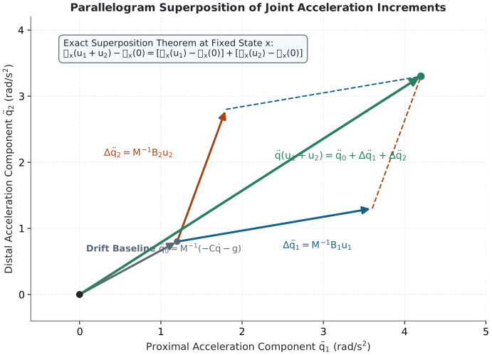
This is the basic superposition statement: at a fixed state \(x\), the incremental effect of each input component on \(\dot x\) is linear and additively separable.
Long description
The vector diagram illustrates vector addition of instantaneous accelerations in joint coordinate space at a single fixed state snapshot. The zero-input drift acceleration vector establishes the baseline coordinate origin. From this point, acceleration increments \(\Delta a_1 = M^{-1}B_1 u_1\) and \(\Delta a_2 = M^{-1}B_2 u_2\) form adjacent sides of a vector parallelogram. The combined acceleration from simultaneous inputs \(u_1 + u_2\) coincides exactly with the diagonal vertex, geometrically proving that state-affine dynamics obey strict additive superposition instantaneously across input channels.For acceleration \(a=a_d+Hu\), subtraction gives \(a-a_d=Hu\): the acceleration increment, not a unique input. Recovering \(u\) also requires a known \(H\), a range-consistent observation, and enough independent input information. If \(H\) has a nontrivial kernel, several inputs give the same increment. Input bounds and noise can further limit inversion. The sign matters: subtracting total acceleration from drift gives \(-Hu\).
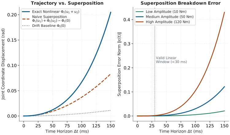
Finite trajectories generally do not add. For the specified linear system \(\dot x=A(t)x+B(t)u+c(t)\), trajectories with the same initial state obey \(x_{u_1+u_2}=x_{u_1}+x_{u_2}-x_0\), with the evolved zero-input baseline counted once. Making the columns of \(G(x)\) linear in state is not enough: \(\dot x=xu\) is bilinear and does not have that input-to-trajectory superposition property.
Long description
The trajectory divergence plot contrasts exact numerical integration of the nonlinear multibody equations against naive addition of independent single-actuator trajectories over time. For short durations under 20 ms, the linear trajectory approximation remains close. Beyond 50 ms, the trajectories diverge sharply because velocities induced by one input alter the centrifugal and Coriolis accelerations that act on the other input channels, causing quadratic and exponential error growth that violates trajectory-level superposition.2.3 Admissible Inputs and a Feasible Reference
The algebra extends to \(u\in\mathbb R^m\), but a physical input set \(\mathcal U(x)\) is generally not a vector space. Bounds, unilateral muscle force, friction and contact reactions may exclude negative inputs, sums of allowed inputs, or zero itself. A component in an algebraic decomposition need not be a separately executable command. For any feasible reference \(u_\star\in\mathcal U(x)\), \[ \begin{aligned} \mathcal F_x(u)-\mathcal F_x(u_\star)&=G(x)(u-u_\star),\\ \Delta\dot{\mathcal X}_{u_\star}&=G(x)\bigl(\mathcal U(x)-u_\star\bigr). \end{aligned} \] The first identity is exact wherever the same model applies. The second is an attainable set relative to that reference, not generally a subspace. Convex combinations remain feasible only when the declared input set is convex; an arbitrary sum does not inherit that property.
For example, let a scalar rotational model have \(a(u)=3+2u\), with \(a\) in rad/s², \(u\) in N·m and gain \(2\) in (rad/s²)/(N·m). Suppose \(1\le u\le2\). Two commands of \(1.5\) are allowed individually, but their sum \(3\) is not. About \(u_\star=1.5\), feasible acceleration increments span \([-1,1]\) rad/s² and total acceleration spans \([5,7]\) rad/s². The formal zero-input acceleration \(3\) is outside this allowed set. It remains useful as an algebraic anchor, but is not a feasible experiment under these bounds.
Thus affinity gives an exact same-state calculation; feasibility determines which calculations describe possible interventions. If changing an input makes a contact slip, open or impact, solve the new mode rather than extending the old affine formula through that event.
The rest of this paper shows that standard rigid-body dynamics models admit the structure (2.1), with the controls entering as generalized forces. In each formulation, the map from those applied loads to acceleration increments is linear at fixed state.
3 Newton–Euler Derivation of Control Affinity and Superposition
We start from the most classical picture: Newton–Euler equations for rigid bodies.
3.1 Single Rigid Body in 3D
Place the body frame at the center of mass. Let \(p\) be its position in a fixed inertial frame, \(R\) map body components into that frame, \(v^B=R^\top\dot p\), and \(\omega^B\) be body angular velocity. Let \(I_B\) be the constant inertia about the center of mass, expressed in body axes. Applied force \(f^{\mathrm{ext},B}\) and moment \(n^{\mathrm{ext},B}\) below exclude gravity; the moment is about the center of mass. Write \(g^B=R^\top g^0\).
The consistent body-frame equations are \[ \begin{aligned} m(\dot v^B+\omega^B\times v^B)&=mg^B+f^{\mathrm{ext},B},\tag{3.1a}\\ I_B\dot\omega^B+\omega^B\times(I_B\omega^B)&=n^{\mathrm{ext},B}.\tag{3.1b} \end{aligned} \] The transport term in the first equation comes from differentiating \(v^B=R^\top\dot p\). A body moving with constant spatial velocity can have a changing body-frame velocity when its axes rotate. At a reference point away from the center of mass, translation and rotation couple through the spatial inertia described below; the decoupled equations above must not simply be reused there.
3.1.1 Identification of Inputs
Choose \(u=(f^{\mathrm{ext},B},n^{\mathrm{ext},B})\in\mathbb R^6\) and state \(x=(p,R,v^B,\omega^B)\). Its kinematics and dynamics are \[ \begin{aligned} \dot p&=Rv^B,\tag{3.3a}\\ \dot R&=R\widehat\omega^B,\tag{3.3b}\\ \dot v^B&=g^B-\omega^B\times v^B+f^{\mathrm{ext},B}/m,\tag{3.4a}\\ \dot\omega^B&=-I_B^{-1}\bigl(\omega^B\times I_B\omega^B\bigr)+I_B^{-1}n^{\mathrm{ext},B}.\tag{3.4b} \end{aligned} \] The drift is the tuple of right-hand sides at \(u=0\), and the input contribution is \[ G(x)u=\left(0_{\mathbb R^3},0_{3\times3},f^{\mathrm{ext},B}/m,I_B^{-1}n^{\mathrm{ext},B}\right).\tag{3.5} \] The rotation-rate component is a tangent matrix in \(T_RSO(3)\), not an arbitrary three-vector. The matrix representation of \(R\) uses nine entries subject to orthogonality constraints, while the physical configuration has six dimensions. This tuple notation avoids a dimensionally inconsistent block matrix.
Thus the vector-field equation on the rigid-body state manifold is \[ \dot x=f(x)+G(x)u.\tag{3.6} \]
The dynamic input blocks are constant for these body-frame wrench inputs. If the force inputs were instead expressed spatially while the velocity remained in body components, their input block would include \(R^\top\). Affinity survives this declared frame change; the numerical input matrix changes.
3.2 Superposition in Inputs for the Single Body
Let us decompose the external wrench \(u\) as a sum
\[ u = u^{(g)} + u^{(c)} + u^{(d)} + \cdots, \tag{3.7} \]
for example:
- \(u^{(g)}\) := wrench generated by a gravity-compensating actuator,
- \(u^{(c)}\) := “control” wrench from a motor,
- \(u^{(d)}\) := disturbance wrench (contact, aerodynamic drag, etc.).
Define
\[ \dot x(u) := f(x) + G(x) u. \tag{3.8} \]
Then
\[ \begin{aligned} \dot x(u) &= f(x) + G(x) \left(u^{(g)} + u^{(c)} + u^{(d)} + \cdots \right) \\ &= f(x) + G(x)u^{(g)} + G(x)u^{(c)} + G(x)u^{(d)} + \cdots. \end{aligned} \tag{3.9} \]
Define
\[ \Delta \dot x^{(i)} := G(x) u^{(i)} \tag{3.10} \]
the incremental contribution of \(u^{(i)}\) to \(\dot x\) relative to the drift. Then
\[ \dot x(u) = f(x) + \sum_i \Delta \dot x^{(i)}. \tag{3.11} \]
This is the Newton–Euler superposition principle for inputs: the instantaneous state derivative is the drift plus a linear sum of contributions from each input.
Again, note the limitation: integrating (3.6) over time, the trajectories \(x^{(i)}(t)\) obtained under each \(u^{(i)}\) do not in general sum to the trajectory under \(u = \sum_i u^{(i)}\).
3.3 Multibody System and Generalized Coordinates
Now consider a multibody system with \(n\) generalized coordinates \(q \in \mathbb{R}^n\) and generalized velocities \(\dot q \in \mathbb{R}^n\). Let \(x = (q, \dot q)\) be the state.
For an open chain or an already reduced system with independent coordinates, the manipulator form is given below. External wrenches treated as inputs must be prescribed loads, not unknown ideal constraint reactions. For closed loops, eliminate the reactions and use the projected input map derived in the constrained-mechanics chapter.
\[ M(q) \ddot q + C(q,\dot q) \dot q + g(q) + d(q,\dot q) = \tau + J^\top(q) f^\text{ext}, \tag{3.12} \]
where:
- \(M(q) \in \mathbb{R}^{n\times n}\) is the symmetric positive definite mass matrix,
- \(C(q,\dot q)\dot q\) collects Coriolis and centrifugal terms,
- \(g(q)\) is the generalized gravity vector,
- \(d(q,\dot q)\) lumps other dissipative terms (e.g., joint friction),
- \(\tau \in \mathbb{R}^n\) is the vector of joint torques (controls),
- \(J(q)\) is the task Jacobian at the contact point(s),
- \(f^\text{ext}\) is the stacked external contact wrench vector.
We can group the right-hand side as a sum of generalized forces:
\[ Q(q,\dot q, u) := \tau + J^\top(q) f^\text{ext}, \tag{3.13} \]
where we think of the controls as
\[ u := \begin{bmatrix} \tau \\ f^\text{ext} \end{bmatrix}. \tag{3.14} \]
3.4 Control-Affine Structure
Solve (3.12) for \(\ddot q\):
\[ \begin{aligned} \ddot q &= M(q)^{-1}\bigl[\tau+J^\top f^\text{ext}\\ &\qquad -C\dot q-g-d\bigr]\\ &= M(q)^{-1}(-C\dot q-g-d)\\ &\quad +M(q)^{-1}\tau+M(q)^{-1}J^\top f^\text{ext}. \end{aligned} \tag{3.15} \] Here \(C\), \(J\), \(g\) and \(d\) are evaluated at the same configuration and velocity as in (3.12).
Define
\[ f(x) := \begin{bmatrix} \dot q \\ M(q)^{-1} \big( - C(q,\dot q) \dot q - g(q) - d(q,\dot q) \big) \end{bmatrix}, \tag{3.16} \]
\[ G_\tau(x) := \begin{bmatrix} 0_{n\times n} \\ M(q)^{-1} \end{bmatrix}, \quad G_f(x) := \begin{bmatrix} 0_{n\times r} \\ M(q)^{-1} J^\top(q) \end{bmatrix}, \tag{3.17} \]
where \(r\) is the dimension of \(f^\text{ext}\). Then
\[ \dot x = \begin{bmatrix} \dot q \\ \ddot q \end{bmatrix} = f(x) + G_\tau(x)\tau + G_f(x) f^\text{ext}. \tag{3.18} \]
Again we see a control-affine system with \(m = n + r\) input channels (\(n\) joint torques and \(r\) external wrench components). At fixed \(x\), the map from \((\tau,f^\text{ext})\) to \(\ddot q\) is affine, and its increment relative to zero input is linear.
3.5 What Changes When Contact Is a Constraint?
For a stationary, smooth bilateral constraint \(\phi(q)=0\), write \(J_c=\partial\phi/\partial q\), \(J_c\dot q=0\) and \(\gamma=\dot J_c\dot q\). Here \(h\) collects the declared input-independent generalized loads on the left of the dynamics: \[ \begin{aligned} M\ddot q+h&=Bu+J_c^\top\lambda,\\ J_c\ddot q&=-\gamma. \end{aligned} \] Assume \(M\) is positive definite and \(J_c\) has independent rows at this state. Eliminating \(\lambda\) gives \[ \begin{aligned} A&=J_cM^{-1}J_c^\top,\\ W&=M^{-1}-M^{-1}J_c^\top A^{-1}J_cM^{-1},\\ a_0&=-Wh-M^{-1}J_c^\top A^{-1}\gamma,\\ \ddot q&=a_0+WBu. \end{aligned} \] This is the constrained analogue of the free-system input map, consistent with the Modern Robotics constrained-dynamics derivation. It applies within the specified regular mode. The inverse \(A^{-1}\) is not available for redundant rows; one must reduce them or specify a consistent generalized solve and reaction allocation.
Since \(J_cW=0\), same-state acceleration differences lie in \(\ker J_c\). Total acceleration need not: its constraint-normal component supplies \(-\gamma\). Also \(WJ_c^\top=0\): a load in the reaction-covector range can change \(\lambda\) without changing acceleration. Ideal reactions do no virtual work on admissible virtual displacements, \((J_c^\top\lambda)^\top\delta q=0\) when \(J_c\delta q=0\). They do not absorb hidden velocity components. The operator \(W\) maps generalized loads to acceleration increments; it is not an ordinary Euclidean projection of arbitrary velocities.
As a checked example, a 2 kg bead on an ideal stationary circular guide of radius 1 m has position \((1,0)\) m and velocity \((0,3)\) m/s. Use \(\phi=(q^\top q-1\,\mathrm{m}^2)/2\), giving \(J_c=(1,0)\) m and \(\gamma=9\) m²/s². With no other loads, a prescribed force \((F_r,F_t)\) produces \[ \ddot q=\left(-9\,\mathrm{m/s^2},\frac{F_t}{2\,\mathrm{kg}}\right). \] Changing \(F_r\) changes the guide reaction, while the required inward acceleration stays \(9\) m/s². Changing \(F_t\) changes tangential acceleration. This example uses a bilateral frictionless guide; a shoe-ground contact must additionally satisfy its normal-force, friction and contact-patch conditions. Moving supports require their time-dependent bias terms and may do work. Impact requires an impulse/momentum model, not this smooth acceleration equation.
3.6 Newton–Euler Superposition Theorem
We can now formalize the Newton–Euler version of superposition.
Let a multibody system with generalized coordinates \(q \in \mathbb{R}^n\) satisfy (3.12). Define the mapping
\[ \Phi_{(q,\dot q)} : \mathbb{R}^n \times \mathbb{R}^r \to \mathbb{R}^n, \quad \Phi_{(q,\dot q)}(\tau, f^\text{ext}) := \ddot q. \]
Then, for each fixed \((q,\dot q)\), the map \[ (\tau, f^\text{ext}) \mapsto \Phi_{(q,\dot q)}(\tau, f^\text{ext}) - \Phi_{(q,\dot q)}(0, 0) \] is linear in \((\tau,f^\text{ext})\).
Proof. From (3.15),
\[ \ddot q = A(q,\dot q) + M(q)^{-1} \tau + M(q)^{-1} J^\top(q) f^\text{ext}, \]
where
\[ A(q,\dot q) := M(q)^{-1} \big( - C(q,\dot q) \dot q - g(q) - d(q,\dot q) \big) \]
depends only on \((q,\dot q)\), not on \((\tau,f^\text{ext})\).
Hence,
\[ \Phi_{(q,\dot q)}(\tau, f^\text{ext}) = A(q,\dot q) + M(q)^{-1} \tau + M(q)^{-1} J^\top(q) f^\text{ext}, \]
and
\[ \Phi_{(q,\dot q)}(0, 0) = A(q,\dot q). \]
Thus,
\[ \Phi_{(q,\dot q)}(\tau, f^\text{ext}) - \Phi_{(q,\dot q)}(0, 0) = M(q)^{-1} \tau + M(q)^{-1} J^\top(q) f^\text{ext}. \]
The right-hand side is a linear map of \((\tau,f^\text{ext})\). ∎
This theorem is the precise incremental superposition statement: for fixed state, acceleration increments relative to the same zero-input baseline superpose linearly.
4 Worked Example: Superposition on a Point-Mass Double Pendulum
Given: a planar point-mass double pendulum, \(m_1=m_2=l_1=l_2=1\), state \(q=(0.5,-0.3)\) rad, \(\dot q=(1.0,0.5)\) rad/s, and two torque vectors \(\tau_1=(2,0)\), \(\tau_2=(0,1)\) N m; gravity is omitted from this pendulum model.
Steps:
- Compute \(M(q)\) via
double_pendulum_mass_matrixand the Coriolis bias \(C(q,\dot q)\dot q\) viadouble_pendulum_coriolis. - Define \(\Phi(\tau)=M(q)^{-1}\big(\tau-C(q,\dot q)\dot q\big)\) and evaluate it at \(\tau=0,\ \tau_1,\ \tau_2,\ \tau_1+\tau_2\).
Result: \(\Phi(0)=(-0.7709,\,2.5089)\), \(\Phi(\tau_1)=(1.8448,\,-1.1359)\), \(\Phi(\tau_2)=(-2.5933,\,9.0483)\), \(\Phi(\tau_1+\tau_2)=(0.0224,\,5.4035)\), so \(\Phi(\tau_1)+\Phi(\tau_2)-\Phi(0)=\Phi(\tau_1+\tau_2)\) to machine precision. Because \(\Phi(\tau)=M(q)^{-1}(\tau-C(q,\dot q)\dot q)\) is affine in \(\tau\) by construction, this identity cannot fail; the numbers above illustrate the theorem’s linear-in-increments statement rather than test it.
Computed by src/affine_control/dynamics.py::double_pendulum_mass_matrix and ::double_pendulum_coriolis; checked against this page by tests/test_worked_example_callouts.py::test_superposition_theorem_double_pendulum.
4.1 Example: Planar Simple Pendulum (Newton–Euler Flavor)
Consider a planar pendulum: point mass \(m\) at end of rigid massless rod length \(l\), pivot at the origin. Let \(q\) be the angle from the vertical, positive counterclockwise. Generalized coordinate \(q \in \mathbb{R}\). We use a sign convention where \(q=0\) is vertical downward.
- Gravity acts along \(-y\) with magnitude \(mg\).
- Applied torque \(\tau\) acts at the pivot.
4.1.1 Equation of Motion
Elementary Newtonian derivation yields:
\[ I \ddot q + mgl \sin q = \tau, \quad I = m l^2. \tag{3.19} \]
Rewrite as
\[ \ddot q = -\frac{g}{l} \sin q + \frac{1}{m l^2} \tau. \tag{3.20} \]
Define state \(x = (q,\dot q)\) and input \(u := \tau\). Then
\[ \dot x = \begin{bmatrix} \dot q \\ -\frac{g}{l} \sin q \end{bmatrix} + \begin{bmatrix} 0 \\ \frac{1}{m l^2} \end{bmatrix} u. \tag{3.21} \]
This is clearly of the form (2.1) with \(m=1\) input.
4.1.2 Superposed Contributions
Suppose we decompose the torque \(u\) as
\[ u = u^{(g)} + u^{(c)}, \tag{3.22} \]
where:
- \(u^{(g)}\) is a “gravity-compensating” component,
- \(u^{(c)}\) is an additional control component.
At some fixed \((q,\dot q)\), the gravitational acceleration term is
\[ \ddot q^{(\text{drift})} = -\frac{g}{l} \sin q. \tag{3.23} \]
The incremental accelerations from each torque component are
\[ \Delta \ddot q^{(g)} = \frac{1}{m l^2} u^{(g)}, \qquad \Delta \ddot q^{(c)} = \frac{1}{m l^2} u^{(c)}. \tag{3.24} \]
The total acceleration is
\[ \ddot q = \ddot q^{(\text{drift})} + \Delta \ddot q^{(g)} + \Delta \ddot q^{(c)}. \tag{3.25} \]
For instance, if \(u^{(g)} = mgl \sin q\) (exact gravity compensation), then
\[ \Delta \ddot q^{(g)} = \frac{1}{m l^2} (mgl \sin q) = \frac{g}{l} \sin q, \tag{3.26} \]
which cancels the drift term (3.23), and we are left with
\[ \ddot q = \frac{1}{m l^2} u^{(c)}. \tag{3.27} \]
This is a very concrete illustration of Newton–Euler superposition: the gravitational component and control component of acceleration add linearly.
5 Lagrangian Derivation of Control Affinity and Superposition
We now re-derive the same structure using Lagrangian mechanics, which highlights the geometric origin of the mass matrix and generalized forces.
5.1 Lagrangian Mechanics and Lagrange–d’Alembert Principle
Let \(Q\) be the configuration manifold, \(q \in Q\) generalized coordinates, \(\dot q \in T_q Q\) generalized velocities. A mechanical system is defined by a Lagrangian
\[ L(q,\dot q) = T(q,\dot q) - V(q), \tag{4.1} \]
with kinetic energy \(T\) and potential energy \(V\).
5.1.1 Kinetic Energy and Mass Matrix
Assume standard mechanical type:
\[ T(q,\dot q) = \frac{1}{2} \dot q^\top M(q) \dot q, \tag{4.2} \]
with \(M(q)\) symmetric positive definite. Then
\[ \frac{\partial L}{\partial \dot q} = M(q)\dot q. \tag{4.3} \]
5.1.2 Generalized Forces
Let \(Q(q,\dot q, t)\) denote the generalized forces, defined by
\[ Q_k = \sum_{j} f_j \cdot \frac{\partial r_j}{\partial q_k}, \tag{4.4} \]
where:
- \(f_j\) are physical forces acting at points with position vectors \(r_j(q)\),
- \(k = 1,\dots,n\) indexes generalized coordinates.
By construction, \(Q\) is linear in the specified point forces. Applied couples contribute their angular-Jacobian transpose mappings as well. Forces already represented through \(V\) must not be counted again in \(Q\); ideal constraints must be reduced or included with multipliers.
5.1.3 Lagrange–d’Alembert Equations
The Lagrange–d’Alembert principle yields
\[ \frac{d}{dt} \frac{\partial L}{\partial \dot q_k} - \frac{\partial L}{\partial q_k} = Q_k, \quad k=1,\dots,n, \tag{4.5} \]
or in vector form,
\[ \frac{d}{dt} \frac{\partial L}{\partial \dot q} - \frac{\partial L}{\partial q} = Q. \tag{4.6} \]
Substituting (4.2) and \(L = T-V\) gives the standard manipulator form:
\[ M(q)\ddot q + C(q,\dot q)\dot q + g(q) = Q. \tag{4.7} \]
Here, \(C\) and \(g\) emerge from the time derivative and the potential term (we do not re-derive them in detail; the important point is that they depend on \((q,\dot q)\) but not on \(Q\)).
5.2 Control Decomposition of Generalized Forces
We now decompose the generalized forces \(Q\) into components induced by distinct physical effects and control channels.
Suppose the physical forces present are:
- internal actuation forces (joint torques, muscle forces, etc.),
- gravity (already represented by \(V\) on the left in this formulation),
- prescribed external loads,
- dissipative forces (viscous friction),
- etc.
Let \(f^{(1)},\dots,f^{(m)}\) denote a collection of force components (or wrenches) we treat as independent. For instance:
- \(f^{(1)}\) = actuator force from motor 1,
- \(f^{(2)}\) = actuator force from motor 2,
- …
- \(f^{(m)}\) = some external load.
By construction of (4.4), the generalized forces are
\[ Q(q,\dot q) = \sum_{i=1}^m Q^{(i)}(q,\dot q), \quad Q^{(i)}(q,\dot q) := \sum_j f^{(i)}_j \cdot \frac{\partial r_j}{\partial q}. \tag{4.8} \]
Define an input vector \(u \in \mathbb{R}^m\) that scales each force component:
\[ f^{(i)} = u_i \bar f^{(i)}, \tag{4.9} \]
where \(\bar f^{(i)}\) is a declared input-independent force pattern with consistent units (for example a fixed direction at a given attachment point). Then
\[ Q^{(i)}(q,\dot q;u_i) = u_i \bar Q^{(i)}(q,\dot q), \tag{4.10} \]
where
\[ \bar Q^{(i)}(q,\dot q) = \sum_j \bar f^{(i)}_j \cdot \frac{\partial r_j}{\partial q}. \tag{4.11} \]
Therefore,
\[ Q(q,\dot q; u) = \sum_{i=1}^m u_i \bar Q^{(i)}(q,\dot q). \tag{4.12} \]
In matrix form,
\[ Q(q,\dot q;u) = B(q,\dot q) u, \tag{4.13} \]
with columns \(B_i(q,\dot q) = \bar Q^{(i)}(q,\dot q)\).
5.3 Control-Affine Lagrangian Dynamics
Substitute (4.13) into the Lagrange equations (4.7):
\[ \begin{aligned} M(q)\ddot q+C\dot q+g&=Bu,\\ \ddot q&=-M(q)^{-1}(C\dot q+g)\\ &\quad+M(q)^{-1}Bu. \end{aligned} \tag{4.14} \] The argument dependence of \(C\), \(g\) and \(B\) is unchanged from (4.7) and (4.13).
Define state \(x=(q,\dot q)\) and vector fields:
\[ \begin{aligned} f(x)&:=\begin{bmatrix}\dot q\\-M(q)^{-1}(C\dot q+g)\end{bmatrix},\\ G(x)&:=\begin{bmatrix}0_{n\times m}\\M(q)^{-1}B\end{bmatrix}. \end{aligned} \tag{4.15} \]
Then
\[ \dot x = f(x) + G(x) u. \tag{4.16} \]
Hence, the Lagrangian equations of motion yield a control-affine system exactly as in (2.1).
5.4 Lagrangian Superposition Theorem
We obtain the Lagrangian analog of the Newton–Euler superposition theorem.
Consider a mechanical system with Lagrangian \(L(q,\dot q)\) and generalized forces of the form \(Q(q,\dot q;u) = B(q,\dot q) u\). Then, for each fixed state \((q,\dot q)\), the mapping \(u \mapsto \ddot q\) given by (4.14) is affine in \(u\), and the incremental effect of \(u\) on \(\ddot q\) (relative to \(u=0\)) is linear in \(u\).
Proof. From (4.14),
\[ \ddot q = - M(q)^{-1} \left( C(q,\dot q)\dot q + g(q) \right) + M(q)^{-1}B(q,\dot q) u. \]
For fixed \((q,\dot q)\), define
\[ A(q,\dot q) := - M(q)^{-1} \left( C(q,\dot q)\dot q + g(q) \right), \quad L(q,\dot q) := M(q)^{-1} B(q,\dot q). \]
Then
\[ \ddot q = A(q,\dot q) + L(q,\dot q) u. \]
Thus the map \(u \mapsto \ddot q\) is affine, and the incremental map
\[ u \mapsto \ddot q - \ddot q\big|_{u=0} = L(q,\dot q) u \]
is linear. ∎
5.5 Example: Planar Pendulum (Lagrangian Derivation)
Re-derive the Newton–Euler pendulum example using Lagrange–d’Alembert.
- Coordinate: \(q\) (pendulum angle).
- Kinetic energy: \(T = \frac{1}{2} m l^2 \dot q^2\).
- Potential energy: \(V = -m g l \cos q\), whose value at \(q=0\) is \(-mgl\); adding \(mgl\) would set that reference value to zero without changing the dynamics.
- Lagrangian: \(L = T - V = \frac{1}{2} m l^2 \dot q^2 + m g l \cos q\).
Compute
\[ \frac{\partial L}{\partial \dot q} = m l^2 \dot q, \quad \frac{d}{dt} \frac{\partial L}{\partial \dot q} = m l^2 \ddot q, \]
\[ \frac{\partial L}{\partial q} = - m g l \sin q. \]
Joint torque \(\tau\) is the generalized force:
\[ Q = \tau. \]
Lagrange–d’Alembert equation:
\[ m l^2 \ddot q - (- m g l \sin q) = \tau \quad\Rightarrow\quad m l^2 \ddot q + m g l \sin q = \tau, \]
which is identical to (3.19). We then repeat the decomposition in (3.22)–(3.27); all linear superposition steps follow directly from the linearity of \(Q\) in \(\tau\).
6 Screw-Theoretic / Spatial Vector Derivation
Screw theory packages translational and rotational quantities into unified twists (velocities) and wrenches (forces/torques). This formalism makes linearity properties especially transparent.
6.1 Twists, Wrenches, and Spatial Inertia
Use body-frame components throughout, with twist \(V=(\omega,v_O)\) and wrench \(F=(n_O,f)\) referenced to the same body-fixed origin \(O\). The dual pairing is power, \(F^\top V=n_O^\top\omega+f^\top v_O\). Let \(c\) point from \(O\) to the center of mass, let \(C=[c]_\times\), and let \(I_C\) be the inertia about the center of mass in the same axes. Then \[ \mathcal I=\begin{bmatrix}I_C+mC^\top C&mC\\-mC&mI_3\end{bmatrix}.\tag{5.3} \] The off-diagonal blocks have opposite signs because \(C^\top=-C\), consistent with Featherstone’s spatial-vector reference. Consequently \(\mathcal I\) is symmetric and \[ \tfrac12 V^\top\mathcal I V=\tfrac12\omega^\top I_C\omega+\tfrac12m\|v_O+\omega\times c\|^2. \] This energy identity independently checks the signs and the parallel-axis term. The spatial momentum is \(h=\mathcal I V\).
Define the force cross-product operator explicitly to avoid coadjoint-sign ambiguity: \[ V\times^*=\begin{bmatrix}[\omega]_\times&[v_O]_\times\\0&[\omega]_\times\end{bmatrix}. \] With constant body-frame spatial inertia, Newton–Euler dynamics are \[ \mathcal I\dot V+(V\times^*)\mathcal I V=F_{\mathrm{all}}.\tag{5.4} \] Here \(F_{\mathrm{all}}\) includes gravity if it has not been separated elsewhere. At fixed complete state the velocity-product term is fixed, so a prescribed wrench increment gives \(\Delta\dot V=\mathcal I^{-1}\Delta F\).
6.2 Multibody Dynamics and Virtual Work
For link \(k\), a consistent body Jacobian gives \(V_k=J_k(q)\dot q\) and \(\dot V_k=J_k\ddot q+\dot J_k\dot q\). Summing kinetic energies yields \(M=\sum_kJ_k^\top\mathcal I_kJ_k\). Eliminating internal joint reactions through virtual work gives the same minimal-coordinate equations as before: \[ M(q)\ddot q+h(q,\dot q)=B(q)u+J_e(q)^\top F_e.\tag{5.6} \] One cannot treat every link twist as an independent coordinate and invert a block of body inertias while ignoring joint constraints. The joint compatibility and internal reactions are essential parts of the articulated system.
6.3 Wrench-to-Load Mapping Is Not a Unique Inverse
For \(V_e=J_e\dot q\), an external wrench applied to the mechanism contributes the generalized load \[ Q_e=J_e^\top F_e, \qquad Q_e^\top\dot q=F_e^\top V_e. \] This is virtual-work duality for the same applied load. It does not assert that total actuator power equals end-effector power while links accelerate, change potential energy, or dissipate energy. Actual actuator torque must satisfy the full dynamics, including those terms. A wrench exerted by the mechanism on its environment has the opposite sign to the environmental wrench applied to the mechanism.
The forward mapping \(F_e\mapsto Q_e\) is linear at fixed configuration. Its inverse may be nonexistent or nonunique. If \(J_e\) has full row rank, then \(J_e^\top\) is injective onto its range, but an arbitrary generalized load need not belong to that range. Rank deficiency permits wrench components in \(\ker J_e^\top\) that have no generalized-load effect. For a real grasp, admissibility also depends on contact type and friction.
For prescribed load components \(F_e=\sum_iF_e^{(i)}\), their acceleration increments are \(M^{-1}J_e^\top F_e^{(i)}\) in the unconstrained or reduced model. Add the drift once. In an unreduced closed-loop model, use its constrained inverse-mass map and solve reactions consistently.
6.4 Example: Spatial Single-Link Actuator
For a free rigid link with prescribed actuator wrench \(F^{\mathrm{act}}=\sum_i u_i\bar F^{(i)}\) and known gravity wrench \(F^{\mathrm{grav}}(R)\), \[ \dot V=\mathcal I^{-1}\left[F^{\mathrm{grav}}-(V\times^*)\mathcal I V\right] +\sum_i\mathcal I^{-1}\bar F^{(i)}u_i. \] The drift depends on orientation through the gravity wrench as well as on \(V\). A function of \(V\) alone is not a complete state description. The formula proves incremental input superposition for this free-body model; a link pinned at a joint must additionally satisfy that joint’s constraints.
7 Cross-Comparison of the Three Formulations
We now summarize and compare the Newton–Euler, Lagrangian, and screw-theoretic versions of the same underlying structure.
7.1 Common Structure
All three approaches lead to equations of the form
\[ \ddot q = f_2(q,\dot q) + H(q,\dot q) u, \tag{6.1} \]
with state \(x=(q,\dot q)\), drift \(f(x)\), and input matrix \(G(x)\) such that
\[ \dot x = f(x) + G(x) u. \tag{6.2} \]
- Newton–Euler: \(M(q)\) arises from summing link inertias; \(H(q,\dot q)\) is \(M(q)^{-1}\) times a matrix that maps torques and external wrenches to generalized forces.
- Lagrangian: \(M(q)\) arises from the kinetic energy metric; \(H(q,\dot q) = M(q)^{-1} B(q,\dot q)\) where \(B\) encodes generalized forces from physical forces.
- Screw theory: the spatial inertia \(\mathcal{I}\) yields \(M(q)\) after coordinate transformation; \(H(q,\dot q)\) is the composition of wrench mappings and \(M(q)^{-1}\).
In each approach, linearity in \(u\) is inherited from:
- The linearity of forces and wrenches in their scalar magnitudes (Newton’s second law is linear in force).
- The linearity of the generalized force mapping from physical forces/wrenches to \(Q\) (via Jacobians).
- The linear solution of the linear system \(M(q)\ddot q = \cdots\) at fixed \(q\).
7.2 What Superposition Does Not Give You
It is essential to stress what we do not get:
- For a general nonlinear mechanical system, if \(x^{(1)}(t)\) solves \(\dot x = f(x) + G(x) u^{(1)}(t)\) and \(x^{(2)}(t)\) solves \(\dot x = f(x) + G(x) u^{(2)}(t)\), then in general \[ x(t) \neq x^{(1)}(t) + x^{(2)}(t) \] A linear system with a common initial state instead uses the evolved-baseline identity given above; the plain sum additionally requires that baseline to vanish. State addition itself requires a compatible vector-space representation.
- Superposition in this paper refers to linear decomposition of applied generalized loads and acceleration increments with respect to input channels at a fixed state. The total acceleration includes its zero-input baseline once.
Still, this local superposition is extremely useful in practice: it allows you to calculate, at each time, how much of the instantaneous acceleration or joint torque is attributable to gravity, inertial coupling, specific actuators, or external loads, etc.
7.3 The Snapshot Principle and Its Time Horizon
At a fixed complete state \(x_0\), a control-affine acceleration model obeys \[ \ddot q(u_1+u_2;x_0)=\ddot q(u_1;x_0)+\ddot q(u_2;x_0)-\ddot q(0;x_0). \] This is an exact affine identity for the chosen model. It does not make force production independent, identify individual muscle forces, or remove state-dependent coupling. Even at one state, the influence of a shoulder torque on club acceleration depends on the whole mass matrix and the active constraints.
Repeating this calculation along an observed trajectory produces a sequence of same-state contributions. Integrating those contributions along that common trajectory can define an accounting quantity, but it is not the same as rerunning the swing with one input removed. A forward intervention changes the state, and therefore subsequent inertia, geometry, force production, and possibly contact mode. Comparing the two constructions is a useful research question, not a reason to label them equivalent.
For a task velocity \(\dot y=J(q)\dot q\), task acceleration also includes \(\dot J\dot q\). For nonzero clubhead velocity \(v_c\), the rate of speed change is \(v_c^\top a_c/\|v_c\|\). Neither instantaneous acceleration nor its norm is a share of the speed already present at impact.
7.4 Coordinate Invariance Has a Defined Meaning
For a smooth, time-independent state diffeomorphism \(y=\psi(x)\) with the same physical inputs, \[ \dot y=D\psi(x)f(x)+D\psi(x)G(x)u. \] Affinity is preserved. The geometric fields are pushed forward; their components and coordinate norms change. For a nonlinear configuration change \(q'=\chi(q)\), coordinate acceleration includes a Hessian term, \[ \ddot q'=D\chi\,\ddot q+D^2\chi[\dot q,\dot q]. \] That term cancels in a same-state acceleration difference, while it belongs to the transformed drift in the total acceleration. Coordinate acceleration by itself is not a tangent vector under arbitrary configuration changes.
A time-dependent state transformation adds \(\partial_t\psi\) to the drift. Changing the input convention also changes the split: if \(u=\alpha(x)+\beta(x)w\), then the new zero-\(w\) drift is \(f+G\alpha\). Thus invariance under state coordinates does not make every choice of passive/active boundary, zero-input intervention, or metric identical. Coriolis terms need not disappear merely because the laboratory axes are inertial; generalized joint coordinates can still have a varying mass matrix.
8 The Modeling Question: Which Inputs and States?
8.1 Activation Dependence Must Be Checked
Nonlinearity in state does not rule out affinity in a declared input. For example, a simplified muscle law \[ F(a,l,\dot l)=aF_{\max}f_l(l)f_v(\dot l)+F_{\mathrm{pass}}(l) \] is affine in activation \(a\) at fixed muscle state, even when the force-length and force-velocity factors are nonlinear. This is a specified constitutive example, not a claim that every muscle model has this form. Pennation, compliant tendon state, history dependence, and the chosen equilibrium formulation need explicit treatment.
If excitation \(e\) is the input and activation \(a\) is a state, the complete state is \((q,\dot q,a,\ldots)\). The simple law \(\dot a=(e-a)/\tau_a\) with constant \(\tau_a>0\) is affine in excitation; instantaneous mechanical acceleration then depends on the activation state, while excitation changes its subsequent evolution. More elaborate activation/deactivation laws must be checked for their actual dependence on \(e\). Calling \(a\) a neural signal or citing state-dependent muscle force is not enough to establish nonaffinity. See the OpenSim activation-dynamics model for a concrete state/input distinction.
8.2 Torque Is a Useful Mechanical Input With Limits
For a specified rigid multibody model, \(M\ddot q+h=B\tau\) is affine in applied torque. This is an exact property of those equations, rather than an arbitrary assumption that biological torque is linear in neural drive. Whether the model describes the measured golfer accurately is a separate empirical question.
A torque envelope \(\mathcal U(x)\) can represent some instantaneous capacity limits. It cannot by itself encode all activation delays, tendon energy, fatigue, or other history unless the necessary internal states are retained. Two histories can arrive at the same joint position and velocity with different feasible future torques. Likewise, zero net joint torque can coexist with muscle co-contraction and nonzero metabolic cost.
Choose the model level for the question: torque-level equations can analyze load transmission; muscle states and constitutive laws are needed to investigate how that torque is generated; neither model alone identifies a neural objective. Geometric constraints, force bounds, uncertainty, and intervention feasibility remain important at every level.
9 Applications and Worked Examples Across Formulations
Long description
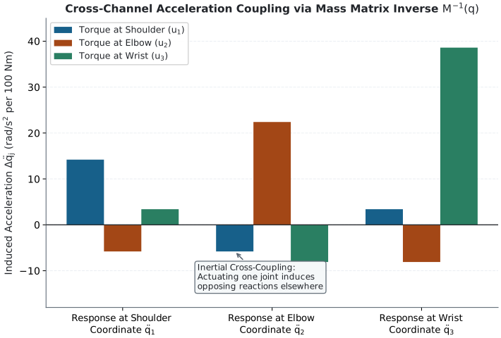
The cross-channel coupling chart details the induced accelerations across joints under individual unit actuator torques. Applying torque solely at the proximal joint produces a direct positive acceleration on the proximal link along with an induced reaction acceleration on the distal link through the off-diagonal mass matrix term \(M_{12}^{-1}\). Conversely, distal torque accelerates the clubhead while exerting an opposing reaction on the proximal segment. This coupling demonstrates why superposition holds per instantaneous force channel even when inertial coordinates are strongly coupled.To make the parallels concrete, we now present two more worked examples: a planar 2R manipulator and a brief screw-theoretic example.
9.1 Example: 2R Planar Robot Arm (Newton–Euler / Lagrangian)
Consider a 2-link planar robot arm. Let \(q_1\) be the first link’s angle from the horizontal and \(q_2\) the second link’s angle relative to the first. Link lengths are \(l_1,l_2\), masses are \(m_1,m_2\), center-of-mass distances along the links are \(c_1,c_2\), and \(I_1,I_2\) are planar inertias about those centers. Gravity acts in \(-y\).
The equations of motion can be written as
\[ M(q) \ddot q + C(q,\dot q)\dot q + g(q) = \tau, \tag{8.1} \]
Use column vectors \(q=(q_1,q_2)^\top\) and \(\tau=(\tau_1,\tau_2)^\top\).
Explicit expressions (standard textbook result, shown here to emphasize structure):
\[ M(q) = \begin{bmatrix} a + 2b \cos q_2 & d + b \cos q_2 \\ d + b \cos q_2 & d \end{bmatrix}, \tag{8.2} \]
where
\[ a = I_1 + I_2 + m_1c_1^2 + m_2(l_1^2+c_2^2), \quad b = m_2 l_1 c_2, \quad d = I_2+m_2c_2^2, \]
as follows by summing both center-of-mass translational energies and both rotational energies. For two uniform unit-length, unit-mass rods at \(q_2=0\), \(c_1=c_2=1/2\) and \(I_1=I_2=1/12\), giving \(M_{11}=8/3\), \(M_{12}=5/6\), and \(M_{22}=1/3\). Omitting the center-of-mass terms changes this physical model.
The Coriolis/centrifugal term is
\[ C(q,\dot q)\dot q = \begin{bmatrix} - b \sin q_2 \, (2\dot q_1 \dot q_2 + \dot q_2^2) \\ b \sin q_2 \, \dot q_1^2 \end{bmatrix}, \tag{8.3} \]
and the gravity vector
\[ g(q) = \begin{bmatrix} (m_1 c_1 + m_2 l_1)g \cos q_1 + m_2 c_2 g \cos(q_1 + q_2) \\ m_2 c_2 g \cos(q_1 + q_2) \end{bmatrix}. \tag{8.4} \]
Rewrite (8.1) as
\[ \ddot q = - M(q)^{-1}\big(C(q,\dot q)\dot q + g(q)\big) + M(q)^{-1}\tau. \tag{8.5} \]
At a fixed \((q,\dot q)\), define:
\[ \ddot q^{(\text{drift})}(q,\dot q) := - M(q)^{-1}\big(C(q,\dot q)\dot q + g(q)\big), \]
\[ L(q,\dot q) := M(q)^{-1}. \]
Then
\[ \ddot q = \ddot q^{(\text{drift})}(q,\dot q) + L(q,\dot q) \tau. \tag{8.6} \]
As before, if we decompose
\[ \tau = \tau^{(g)} + \tau^{(c)} + \tau^{(d)}, \tag{8.7} \]
corresponding to gravity compensation, control, and disturbance, we have
\[ \ddot q = \ddot q^{(\text{drift})} + L(q,\dot q) \tau^{(g)} + L(q,\dot q) \tau^{(c)} + L(q,\dot q) \tau^{(d)}. \tag{8.8} \]
Each term \(L(q,\dot q) \tau^{(i)}\) is the instantaneous acceleration contribution of the corresponding torque component.
9.1.1 Lagrangian Viewpoint
From the Lagrangian viewpoint, the same equations arise from
- \(L = T - V\) with appropriate kinetic and potential energy expressions,
- generalized forces \(Q = \tau\).
The key distinction is interpretive: Lagrangian mechanics frames \(M(q)\) as a metric on \(Q\), and \(g(q)\) as the gradient of a potential. But the linearity in \(u\) (here \(u=\tau\)) is identical to the Newton–Euler derivation.
9.2 Example: Planar End-Effector Wrench
For the same 2R arm, take \(f_e=(f_x,f_y)^\top\) to be a force applied by the environment to the end effector, with no applied couple. Differentiating its position gives \[ J_e=\begin{bmatrix} -l_1\sin q_1-l_2\sin(q_1+q_2)&-l_2\sin(q_1+q_2)\\ l_1\cos q_1+l_2\cos(q_1+q_2)&l_2\cos(q_1+q_2) \end{bmatrix}. \] The generalized load of this force is \(Q_e=J_e^\top f_e\), and \(Q_e^\top\dot q=f_e^\top\dot p_e\). With applied joint torque \(\tau_{\mathrm{act}}\), the dynamics are \[ \ddot q=a_d+M^{-1}\tau_{\mathrm{act}}+M^{-1}J_e^\top f_e. \] Separate prescribed load components add through \(M^{-1}J_e^\top\) at the same state. Actuator and environmental loads must not be counted twice as if an action-reaction pair were two forces on the same system. If \(f_e\) is instead an unknown reaction enforcing a rigid contact, solve that contact constraint; it cannot be varied freely as an independent input.
10 Conclusions
We have shown, in three formulations (Newton–Euler, Lagrangian, screw-theoretic), that:
- Multibody mechanical systems with actuation via generalized forces admit control-affine dynamics of the form \[ \dot x = f(x) + G(x) u, \] where \(x = (q,\dot q)\) and \(u\) parameterizes joint torques and/or external wrenches.
- For each fixed state \(x\), the mapping \(u \mapsto \dot x\) (or \(u \mapsto \ddot q\)) is affine, and the incremental dependence on \(u\) (relative to \(u=0\)) is linear.
- This yields a rigorous superposition principle for inputs: the instantaneous contributions of different input channels (actuators, gravity compensation, disturbances, contact forces) to generalized accelerations and wrenches add linearly.
- The principle is identical in essence across Newton–Euler, Lagrangian, and screw-theoretic settings; they differ in how the mass matrix and generalized forces are constructed, not in the linearity structure.
At the same time, we emphasized that trajectory-level superposition is false in general for nonlinear systems. Superposition here is a local statement about the linear structure of forces and wrenches and their mapping into acceleration increments at a given state.
This clarified view of superposition is particularly valuable for:
- decomposition of motion into gravity, inertial coupling, external, and control contributions;
- design and analysis of gravity compensation and feedforward controllers;
- counterfactual simulations (e.g., “what would the motion be under zero gravity?”, “what if a particular actuator were disabled?”);
- screw-theoretic modeling of force transmission and manipulability.
For golf, the decomposition supplies a model-conditioned acceleration budget. It does not by itself assign unique causal shares of clubhead speed, muscle effort, or metabolic expenditure. A forward intervention, an observed correlation, and an algebraic same-state partition answer different questions.
Velocity-quadratic inertial terms may become large in some configurations, but a large drift-to-input ratio does not prove attraction, negligible steering, or loss of reachability. The system \(\dot x=x+u\) can have a large drift compared with bounded input while nearby uncontrolled states separate exponentially. Evaluate finite-horizon sensitivities, feasible input directions, a declared metric, and the delivered impact state rather than inferring stability from a magnitude ratio.
11 Tests of the Argument
Intervention Feasibility. A mathematical torque clamp is not instantaneous muscle deactivation. State whether passive tissue, activation, grip contact, and prescribed base motion remain in the model, and check feasibility of the resulting loads. This determines what the counterfactual can explain.
Causal Identification. The same input can affect several links through inertia and reactions; different muscle inputs can produce the same net torque. The decomposition must be accompanied by an identification argument and a sensitivity analysis before it supports an empirical causal claim.
Feedback and Outcome Sensitivity. Perturbation direction, remaining time, feedback pathways, force limits, and the sensitivity of impact outcomes all matter. A small attainable correction can matter greatly for face orientation even when it is small relative to total acceleration. A drift-to-input magnitude ratio alone cannot determine whether feedback matters.
Falsification and Alternative Explanations. Compare predictions across plausible inertial parameters, grip compliance, and muscle allocations that fit the observations. If the claimed advantage disappears under those alternatives, report it as model-sensitive. Test proposed interventions against measured outcome changes rather than promoting a convenient algebraic split into a universal instruction.
12 Scope and Limitations
The exact result is incremental superposition in a declared control-affine mechanical model at one complete state. It is compatible with nonlinear state dynamics and finite-time interaction. It does not assume that neural drive maps linearly to torque, that high-speed models are automatically more accurate than quasi-static models, or that a torque-level description identifies individual muscles. Model validation, parameter identification, and human outcome evidence remain separate requirements.
13 Revision History
2026-09-22: Clarified feasible-input superposition and constrained task authority (#4419).
2026-09-08: Standardized cross-article category metadata and link targets (#4302).
2026-09-05: Refined long-form mechanics, control, and impact arguments (#4153).
2025-11-28: Initial publication of multi-formalism superposition derivation.
14 References
The derivations above use virtual work, rigid-body energy, and fixed-state linear algebra. These references develop the underlying mechanics and control formulations; they are not empirical validation of a particular golf intervention.
- Featherstone, R. Rigid Body Dynamics Algorithms. Springer, 2008.
- Murray, R. M., Li, Z., Sastry, S. S. A Mathematical Introduction to Robotic Manipulation. CRC Press, 1994.
- Spong, M. W., Hutchinson, S., Vidyasagar, M. Robot Modeling and Control. Wiley, 2005.
- Bullo, F., Lewis, A. D. Geometric Control of Mechanical Systems. Springer, 2004.
- Greenwood, D. T. Advanced Dynamics. Cambridge University Press, 2003.
Citation
@online{olson2025,
  author = {Olson, Dieter},
  title = {Superposition in {Affine} {Control} {Systems} via
    {Newton–Euler,} {Lagrangian,} and {Screw-Theoretic} {Formulations}},
  date = {2025-11-28},
  url = {https://affinedrift.com/articles/superposition.html},
  langid = {en},
  abstract = {This article develops a rigorous derivation of input
    superposition for finite-dimensional mechanical systems whose
    dynamics are affine in control. Comparing Newton–Euler, Lagrangian,
    and screw-theoretic formulations, it proves that while trajectories
    in state space do not superpose due to nonlinearities, the
    contributions of distinct input channels to generalized forces and
    accelerations strictly superpose.}
}