Drift, Control Capacity and Golf-Swing Correction
These entries remain visible until evidence-backed adjudication changes their governed status.
- Responded / High: Critique: Dimensional Inconsistency of the Drift-Control Ratio (
crit-dimensional-inconsistency-dcr) - Responded / High: Critique: Drift-Control Ratio (Formalism Overreach) (
crit-lie-bracket-formalism-overreach) - Responded / Medium: Critique: Normative Ambiguity of Drift (The "Good Drift" Hypothesis) (
crit-normative-ambiguity-drift) - Responded / High: Critique: Planar Blindness in DCR and Control Cone Analysis (
crit-planar-dcr-blindness) - Responded / High: Critique: Precision vs. Gross Control (The "locked-in" Fallacy) (
crit-precision-gross-control)
The drift-control ratio (DCR) compares modeled acceleration under a declared zero-input baseline with the largest acceleration contribution available from a declared input set. It can help describe a state of the golfer-club model, but it does not establish that control has disappeared, that stored energy is being used efficiently, or that a shot can be corrected before impact. Those questions involve direction, time, activation, geometry, contact and the outcome being corrected.
This article derives the distinction between available capacity and realized input, explains why quadratic velocity terms need not produce monotone drift growth, and shows how coordinates and metrics change the reported number. Exact examples connect those issues to finite-horizon reachability and event-time sensitivity. No calibrated golf-swing growth factor is established here. The earlier numerical downswing-growth claim is withdrawn because no complete parameter set, state history, input history and reproducible model result supported it. The governed analytic and synthetic validation cases remain useful evidence about mathematical limits, with golfer-level effects left to measurement.
1 Scientific Trust Panel
1.1 DCR Is Not a Reachability Certificate
Qualification: Governed — scope-bounded
Claim ID: ad-dcr-001
Evidence class: Analytical Counterexample
Critique status: Adjudicated
Reviewed: 2026-08-28 at 524c28926f364631ed06b15be9c6fdf440acce64
Plain-language summary: A large DCR may flag a modeled acceleration imbalance worth investigating. It does not prove that a golfer is locked-in or that a future correction is unavailable.
Technical claim (Bounded): Within a declared model, DCR compares the magnitudes of modeled drift acceleration and the largest modeled input acceleration in chosen coordinates. DCR alone does not prove or determine finite-horizon reachability, path-correction authority, an impact outcome, or a locked-in golfer state.
Population: Declared dynamical models and admissible input sets; no golfer population is inferred.
Valid conditions:
- Drift and input accelerations are evaluated at the same state in the same coordinates.
- The admissible input set, weighting, norm, and regularization are declared.
Uncertainty (Unquantified): Model-form, input-set, coordinate, norm, parameter, and measurement uncertainty are not quantified by the scalar ratio.
Limitations:
- DCR depends on the declared state, input set, projection, weighting, norm, and regularization.
- The analytical counterexample is not a participant-level golf validation or a coaching prescription.
- Adjudication here applies to this bounded reachability claim; separately listed critiques retain their own ledger status.
Falsifier:
- For the scalar system x_dot = d + u with constant d, fixed horizon T, fixed bound |u(t)| <= U and no state constraints, changing d changes the reachable-interval width 2 U T.
- A scalar DCR value alone uniquely determines a finite-horizon reachable set across admissible systems.
Software provenance:
- D-sorganization/AffineDrift@524c28926f364631ed06b15be9c6fdf440acce64 — src/affine_control/reachability.py (SHA-256 783935d0252a3e384ce9a4f3ba07487738693cd43fb289fa090336332fd75191)
Data provenance: No participant dataset is used; the governing evidence is an exact analytical constant-drift counterexample and its executable regression test.
Next validation gate: Run preregistered finite-horizon, three-dimensional golfer-club perturbation studies with declared controls, uncertainty, and impact outcomes.
This page’s registered claim(s) are documented in the Claim Ledger:
Reachability in More Detail
A moving golfer and club already have velocity, configuration and tissue state. New muscle commands act on that existing state. DCR asks how large one modeled acceleration contribution is compared with the capacity of another; it does not divide a swing into percentages supplied by physics and the golfer.
Imagine a canoe in a uniform current. Increasing the current shifts the possible endpoints downstream. With the same paddling limits and travel time, it need not reduce the range of endpoints around that shifted center. A real river can have banks and changing flow; a real swing has changing geometry, muscle capacity and an impact event. Those details decide which corrections are possible.
DCR alone does not establish which endpoints remain reachable.
A small available correction can matter if the required adjustment is small. Conversely, a large acceleration capacity in the wrong direction or with too little time remaining can be ineffective. A useful investigation therefore reports the desired change in club delivery alongside the forces, directions and time available to make it.
Questions About Noise, Face Control and Impedance
Does less realized torque imply less noise? Harris and Wolpert proposed a model in which control-signal noise influences eye and arm movement planning. It does not measure DCR or demonstrate that golfers minimize noise by maximizing that ratio. A capacity denominator is also different from the command producing noise. Compare complete policies under the same noise and task model. Primary paper.
Can face control remain effective when path control is limited? This is a spatial, task-dependent hypothesis. Forearm motion, wrist configuration, grip and shaft deformation contribute to club orientation; a small isolated axial inertia does not establish the control authority of the coupled chain. The planar model below cannot calculate those omitted effects.
Does impedance provide another form of control? Activation, tendon mechanics and feedback can change the response to a perturbation. A held controller can be included in a declared baseline, but that does not make it mechanically passive or eliminate its energy cost. Moving references and changing stiffness can supply energy. See the corrected passive-control chapter.
These are authored modeling questions. They are not quotations from unnamed critics or evidence that any one mechanism explains expert golf.
The drift-control ratio compares two modeled accelerations. One is what the club and golfer do with zero input. The other is the most the allowed inputs could add.
A Model Number
The ratio depends on the chosen model, coordinates, and input limits. It does not measure muscle effort. It does not show that control has vanished or that energy is used well.
Size Is Not Reach
Think of a canoe in a steady current. A stronger current shifts where you can end up. It need not shrink the range of places you can reach. A real swing has changing geometry, muscle limits, and an impact.
What Is Withdrawn
The earlier growth figure for the downswing is withdrawn. No complete model run supported it. The exact and synthetic examples show mathematical limits only, not golfer results.
2 Introduction
The central investigation is how a golfer prepares and guides a rapidly moving coupled system. The same motion can be compatible with different combinations of active torque, elastic response and feedback. A useful account should predict what changes when an input, initial state or constraint changes, and should connect that prediction to a measured club-delivery outcome.
The control-affine form
\[ \dot x=f(x)+G(x)u \]
organizes that calculation once the state and input have been specified. Here drift means evolution under the selected zero-input convention. It is not a direct measurement of physiological passivity, stored energy, intention or effort. A high-speed state may have large velocity-dependent accelerations, but no universal transition from active control to autonomous motion follows from speed alone.
DCR is a local magnitude diagnostic. A forward zero-torque counterfactual instead integrates a changed input condition from a declared initial state. A reachable-set calculation explores a family of admissible inputs over time. These tools answer related questions and require different evidence.
3 System Modeling: The 3-Link Arm–Forearm–Club Model
Consider a fixed-base, open, planar chain with three rigid links. Let \(q_1\) be the first link’s angle from a fixed axis, and \(q_2,q_3\) the relative elbow and distal hinge angles. These are model coordinates, not a complete anatomical description of shoulder, elbow, forearm and wrist motion. The lengths are \(\ell_i\), masses \(m_i\), center-of-mass distances \(r_i\) along each link, and planar center-of-mass inertias \(I_i\). All must be specified before a numerical swing result can be reproduced.
3.1 Forward Kinematics
With \(\theta_i=\sum_{j=1}^i q_j\), a modeled clubhead point is
\[ p(q)=\begin{bmatrix} \ell_1\cos q_1+\ell_2\cos(q_1+q_2)+\ell_3\cos(q_1+q_2+q_3)\\ \ell_1\sin q_1+\ell_2\sin(q_1+q_2)+\ell_3\sin(q_1+q_2+q_3) \end{bmatrix}. \]
Write \(J=\partial p/\partial q\). Differentiation gives both
\[ \dot p=J(q)\dot q, \qquad \ddot p=J(q)\ddot q+\dot J(q,\dot q)\dot q. \]
The curvature term is essential. A unit-radius point with angle \(q=t\) has zero angular acceleration but Cartesian acceleration \((-\cos t,-\sin t)\). Thus projecting joint acceleration with \(J\) alone does not recover the total task acceleration. If \(\ddot q=a_d+B_a u\), the Cartesian decomposition is
\[ a_{d,p}=J a_d+\dot J\dot q, \qquad B_{a,p}=J B_a. \]
A joint-space projection and a Cartesian-acceleration DCR are different declared diagnostics. The latter includes the curvature term in its drift numerator.
3.2 Lagrangian Dynamics
For this open-chain model, center-of-mass positions follow by replacing the last link length in each partial chain with \(r_i\). Define
\[ T=\frac12\sum_{i=1}^3\left(m_i\|J_{c,i}(q)\dot q\|^2+I_i\dot\theta_i^2\right) =\frac12\dot q^T M(q)\dot q, \qquad U_g=\sum_{i=1}^3m_i g_0 y_{c,i}(q). \]
Here \(g_0>0\) is gravitational acceleration and the fixed vertical axis points upward. These definitions determine the mass matrix and potential; they do not determine a motion or an input history. With \(v=\dot q\), the equations are
\[ M(q)\dot v+c(q,v)+g(q)=B(q)u,\qquad g=\nabla U_g. \]
The vector \(c=Cv\) is quadratic in velocity for this rigid, time-independent Lagrangian model; a particular matrix \(C\) is not unique. The standard manipulator equations and their assumptions are developed in MIT’s multibody notes.
Assume independent coordinates and positive-definite \(M\). Then
\[ a_d=-M^{-1}(c+g),\qquad B_a=M^{-1}B, \]
\[ f(x)=\begin{bmatrix}v\\a_d\end{bmatrix}, \qquad G(x)=\begin{bmatrix}0\\B_a\end{bmatrix}, \qquad x=(q,v). \]
Three independent ideal joint torques correspond to \(B=I_3\) and full actuation of the three modeled acceleration coordinates. Bounds on those torques restrict achievable acceleration; they do not by themselves remove an input channel or change the six-dimensional state-space dimension. A deliberately passive hinge, excitation-driven muscle model or flexible shaft requires a different input map and possibly additional states.
A zero excitation command does not instantly erase activation or tendon strain. Likewise, writing \(u=u_0(x,t)+w\) moves \(G u_0\) into a baseline only after declaring that held policy and its shifted admissible set for \(w\). Drift is unique for a fixed vector field and input origin; it is not invariant under arbitrary changes of that modeling convention. Muscle and shaft state connect this bookkeeping to the muscle-force and flexible-shaft chapters.
3.3 Quadratic Velocity Terms and Their Limits
At a fixed configuration and fixed velocity direction \(\bar v\), scaling speed by a dimensionless \(\lambda\) gives
\[ c(q,\lambda\bar v)=\lambda^2c(q,\bar v), \qquad W a_d(q,\lambda\bar v)=\lambda^2 A+b, \]
where \(A=-WM^{-1}c(q,\bar v)\) and \(b=-WM^{-1}g(q)\). The triangle inequality gives
\[ \|\lambda^2 A+b\|\leq\lambda^2\|A\|+\|b\|. \]
If \(A\neq0\), the numerator divided by \(\lambda^2\) tends to \(\|A\|\) as \(\lambda\to\infty\). That asymptotic statement does not imply monotone growth over a finite downswing. Gravity and the velocity term may cancel at intermediate speeds; \(A\) may vanish in a chosen direction or projection; a constant-inertia model can have \(c=0\). Configuration, velocity direction, weights and admissible muscle forces also vary along a real trajectory.
A capacity denominator remains constant under this speed scaling only if \(M\), \(B\), \(W\) and the input set are held fixed. Muscle force-velocity behavior can change the admissible set, but shortening, lengthening, activation and geometry must be modeled together. The magnitude of the realized torque need not equal capacity or decline with speed. Therefore neither an inevitable DCR blow-up nor a specific downswing growth factor follows from quadratic velocity dependence alone.
4 Drift-Control Ratio (DCR)
In a declared acceleration space, the canonical definition is
\[ \mathrm{DCR}_{W,\mathcal U}(x)= \frac{\|W a_{\mathrm{drift}}(x)\|} {\sup_{u\in\mathcal U(x)}\|W B_a(x)u\|+\varepsilon}. \]
The drift and input effects are evaluated at the same state. \(W\) selects/scales the coordinates or task directions; the norm and admissible input set \(\mathcal U(x)\) are part of the definition. In the equations above, \(a_{\mathrm{drift}}=a_d\). The denominator describes available capacity, not the current command. See the Mathematical Notation Reference.
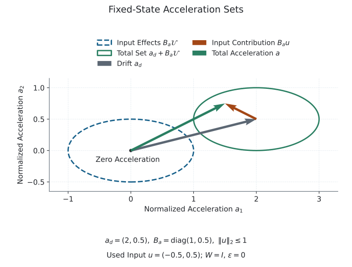
Long Description
At one fixed state, use normalized acceleration coordinates, the Euclidean norm, \(W=I\) and \(\varepsilon=0\). Declare \(a_d=(2,0.5)\), \(B_a=\operatorname{diag}(1,0.5)\) and the unit disk \(\mathcal U=\{u:\|u\|_2\leq1\}\). The blue ellipse is the input-only set \(B_a\mathcal U\), centered at zero acceleration. The green ellipse is the total acceleration set \(a_d+B_a\mathcal U\), translated by drift. The origin is zero acceleration, not the system’s current state. The admissible input \(u=(-0.5,0.5)\) supplies \(B_a u=(-0.5,0.25)\), giving total acceleration \((1.5,0.75)\). Available acceleration capacity is one, so DCR is \(\sqrt{4.25}\) in this stipulated example. The diagram supplies no state trajectory, finite-time reachable set or measured golfer result.Let \(d=\|Wa_d\|\), \(c_{\max}=\sup_{u\in\mathcal U}\|WB_a u\|\) and \(r=\|WB_a u_{\mathrm{used}}\|\). Assume the capacity is finite. The policy-dependent drift-to-realized-input ratio is
\[ \mathrm{DIR}_W=\frac{d}{r+\varepsilon},\qquad \mathrm{DCR}_{W,\mathcal U}=\frac{d}{c_{\max}+\varepsilon}. \]
For an admissible realized input and the same nonnegative regularizer, \(r\leq c_{\max}\), so DIR is at least DCR whenever both are defined. Small realized input can make DIR large while substantial capacity remains unused. For example, \(d=3\), \(c_{\max}=1\), \(r=0.2\) and \(\varepsilon=0\) give DCR \(3\) and DIR \(15\). Neither number identifies why that policy used a small input.
The regularizer has the same units as the weighted acceleration norm. It must change consistently when units or scaling change. For \(c_{\max}>0\),
\[ \mathrm{DCR}_{\varepsilon} =\frac{\mathrm{DCR}_{0}}{1+\varepsilon/c_{\max}}. \]
Thus a regularized value of 10 means \(d=10(c_{\max}+\varepsilon)\), not necessarily \(d=10c_{\max}\). With \(d=11\), \(c_{\max}=1\) and \(\varepsilon=0.1\) in common units, the regularized ratio is 10 while the unregularized ratio is 11.
Report zero capacity explicitly. If \(c_{\max}=0\), positive \(d\) has no finite unregularized ratio and \(d=0\) gives an undefined \(0/0\). A positive regularizer returns a finite display value, but it creates no physical capacity. State the regularizer and flag this condition rather than interpreting the number as control authority. Unknown input bounds likewise cannot be replaced by a physiological estimate inferred from motion alone.
4.1 Dimensional Analysis and Norm Dependence
The full state derivative combines coordinate velocities and accelerations. An unscaled Euclidean norm of those blocks mixes unlike units. Restricting the ratio to accelerations removes that particular inconsistency; it does not make every coordinate choice or metric equivalent. Mixed rotational/translational coordinates require declared scaling, and rank-deficient \(W\) intentionally discards some directions.
4.1.1 A Reproducible Norm Comparison
Take drift \((3,4)\) and the admissible input effects \(\{(u,0):|u|\leq2\}\), in common acceleration units, with no regularization. The Euclidean ratio is \(5/2=2.5\); the infinity-norm ratio is \(4/2=2\). With positive-definite weight matrix \(H=\operatorname{diag}(1,9)\) and \(\|a\|_H=\sqrt{a^THa}\), it is \(\sqrt{153}/2\approx6.185\). These numbers describe the same state and input set under different metrics. They are not estimated values for golfers.
A scalar directional ratio can also differ because it asks a different question. In this example, the second coordinate has nonzero drift but zero input capacity. The overall Euclidean capacity is nevertheless positive. A large denominator in one direction cannot supply an unavailable correction in another.
4.1.2 Force Metrics and Inertia Weighting
For a Euclidean outer norm, let \(a=M^{-1}\tau\) and let the acceleration metric be \(H=W^TW\). Transporting it to generalized forces gives
\[ \|Wa\|^2=\tau^T M^{-T}H M^{-1}\tau. \]
The corresponding force metric is \(M^{-T}HM^{-1}\), not automatically the identity. For \(M=\operatorname{diag}(1,10)\), drift force \((1,1)\) and input forces \((u,0)\) with \(|u|\leq1\), the unweighted force ratio is \(\sqrt2\), whereas the unweighted acceleration ratio is \(\sqrt{1.01}\). Applying the transported force metric recovers the acceleration result.
For an inertia-weighted acceleration norm, \(H=M\), the force metric is \(M^{-1}\). This weighting incorporates inertia, but \(a^TMa\) is not kinetic energy: acceleration has different units from velocity. It is not uniquely preferred for every task, and it does not automatically solve comparisons across joints, coordinate charts or omitted directions.
4.1.3 Coordinate Changes and Reporting
A nonlinear coordinate change \(z=\psi(q)\) obeys
\[ \ddot z=D\psi(q)\ddot q+D^2\psi(q)[\dot q,\dot q]. \]
The second term contains the Hessian of the coordinate map. Ordinary coordinate acceleration therefore does not transform as a tangent vector. In the free scalar system \(\ddot q=u\), the original drift acceleration is zero. On the valid chart \(q>0\), choose \(z=q^2\). Then
\[ \ddot z=2\dot q^2+2qu. \]
At \(q=1\), \(\dot q=1\) and \(|u|\leq1\), the unregularized scalar ratio in \(q\) is zero, while in \(z\) it is one. The physical motion and controls have not changed; the measured coordinate acceleration has. A tensorial acceleration construction would require a declared connection and corresponding decomposition. That is a different specification from silently applying a Euclidean norm to chart accelerations.
For a constant invertible linear change \(z=Lq\), the Hessian term vanishes. Transporting the metric as \(H_z=L^{-T}H_qL^{-1}\) preserves the norm; changing units also requires consistent input and regularizer units. Report the chart/frame, physical output, weights, norm, input set, baseline and regularization. Growth ratios do not remove these dependencies, and a growth ratio with a zero initial numerator is undefined.
5 DCR and Reachability: What the Scalar Does Not Prove
For the control-affine system \(\dot x=f(x)+G(x)u\), keep three objects distinct:
The drift-affected instantaneous velocity set \(f(x) + G(x)\mathcal{U}(x)\).
The input-only control-effect set \(G(x)\mathcal{U}(x)\).
The finite-horizon reachable set
\[ \mathcal{R}(T;x_0)=\{x(T):x(0)=x_0,\;u(t)\in\mathcal U(x(t)),\;0\leq t\leq T\}. \]
Admissibility must also include any state, contact and input-rate constraints in the chosen model. At a fixed state, adding drift translates the first set and leaves the second unchanged. Over time, state dependence in \(f\), \(G\) and \(\mathcal U\) can translate, rotate, stretch or contract reachable outcomes. DCR alone does not determine finite-horizon reachability.
For a dual direction \(p\), the instantaneous support function is
\[ H(x,p)=p^T f(x)+\sup_{u\in\mathcal U(x)}p^T G(x)u. \]
The first term supplies drift support in that direction and the second supplies control support. Their separate norms cannot recover this directional information or its propagation to impact. A set with the same largest control-effect norm can have very different support along the required correction direction.
5.1 Executable Constant-Drift Counterexample
For \(\dot x=d+u\) with constant \(d\), \(|u(t)|\leq\bar u\) and no state constraints,
\[ \mathcal R(T;x_0)=[x_0+(d-\bar u)T,\;x_0+(d+\bar u)T]. \]
Its center is \(x_0+dT\) and its width is \(2\bar uT\), independent of \(d\). With \(x_0=0\), \(\bar u=1\) and \(T=1\), zero drift gives \([-1,1]\) and \(d=100\) gives \([99,101]\). The DCR-like first-order magnitude ratio rises from 0 to 100 while the reachable width remains 2. The checked implementation is src/affine_control/reachability.py::constant_additive_drift_interval, exercised by tests/test_dcr_reachability_contract.py.
The word like matters: \(x\) is a scalar first-order state here, whereas the canonical mechanical DCR is defined in an acceleration space. The example refutes the general inference from drift/input magnitude to reachable-set shrinkage. It does not claim that a golf swing has constant drift. A fixed target near the original center can become unreachable even though the width is unchanged; translation and loss of width are different effects.
6 Worked Example: Reachable Width Is Independent of Drift
Given: \(\dot x=d+u\), \(x_0=0\), \(|u(t)|\leq\bar u=1\), \(T=1\); compare \(d=0\) against \(d=100\).
Steps:
- Call
constant_additive_drift_interval(initial_state=0.0, drift=d, control_bound=1.0, horizon=1.0)for \(d=0\) and \(d=100\).
Result: \(d=0\Rightarrow[-1,1]\); \(d=100\Rightarrow[99,101]\) — the interval’s width stays \(2\) in both cases although the DCR-like magnitude ratio rises from \(0\) to \(100\).
Computed by src/affine_control/reachability.py::constant_additive_drift_interval; checked against this page by tests/test_worked_example_callouts.py::test_dcr_reachable_width_independent_of_drift.
6.1 Interactive: DCR Through a Phase
This widget compares two declared scalar systems that share the same instantaneous DCR at the start of the phase: an additive-drift system (\(\dot x=b+u\)) and a state-dependent-drift system (\(\dot x=ax+u\)), both built from src/affine_control/reachability.py::LinearScalarSystem. Dragging the phase slider evolves each system along its own zero-input drift trajectory and recomputes instantaneous_scalar_dcr at that state, so you can watch the ratio hold flat for one system and grow for the other. The reachable-interval width at the declared horizon, from scalar_linear_reachable_interval, is computed once from the starting state and does not track either curve.
■ Additive drift · ■ State-dependent drift · chart vertical axis maximum: —
| Quantity | Additive drift | State-dependent drift |
|---|---|---|
| Instantaneous DCR now | — | — |
| Reachable interval at $T$ | — | — |
| Reachable-interval width | — | — |
Sampled values across the phase (data table)
| Phase time $t$ | DCR, additive | DCR, state-dependent |
|---|
This is an exploratory model output, not a golfer measurement: the two systems are declared mathematical constructions chosen to hold DCR fixed at the start of the phase, the same construction checked in tests/test_dcr_event_sensitivity_protocol.py::test_state_dependent_drift_breaks_any_dcr_to_reachable_width_mapping.
6.2 What a DCR Threshold Means
Without regularization, a DCR of 10 means the reported drift norm is ten times the largest input-effect norm in the selected acceleration metric. With positive regularization, the exact relation is \(d=10(c_{\max}+\varepsilon)\). Nothing discontinuous occurs at that number. It is not an accessibility, saturation or reachable-set threshold.
Whether correction is sufficient depends on the requested change, remaining horizon, state-dependent admissible control set, task metric, model and measurement uncertainty, and impact-event outcome with its acceptable tolerance. An acceleration norm cannot supply all of those declarations.
DCR also does not predict separation from a forward Zero Torque Counterfactual (ZTCF). That separation requires integrating the declared intervention with its diverging state, contact rules and held-controller assumptions. The original trajectory’s instantaneous drift is not the future counterfactual trajectory.
7 Short-Time Sets and Finite-Time Correction
As \(\Delta t\to0^+\), the unscaled reachable set approaches the initial state. For smooth \(f,G\), a fixed compact convex input set, unconstrained local motion and measurable admissible inputs, the first-order rescaled reachable sets have the limit
\[ \lim_{\Delta t\to0^+}\frac{\overline{\mathcal R(\Delta t;x)}-x}{\Delta t} =f(x)+G(x)\mathcal U, \]
in the Hausdorff sense. Closure accounts for endpoint limits. A Taylor expansion makes the reason visible: the leading displacement is drift times \(\Delta t\) plus the input map times the time integral of \(u\); the average input belongs to the convex set. Local uniform bounds make the remainder smaller than order \(\Delta t\).
Convexity cannot be silently dropped. In \(\dot x=u\), with instantaneous inputs restricted to \(\{-1,1\}\), half a short interval at each input produces zero net displacement. The rescaled endpoints therefore include zero, although the instantaneous velocity set does not. Arbitrarily fast switching gives the convexified leading-order set. Input-rate restrictions, a state-dependent input set or an active state boundary need their own analysis; the displayed assumptions do not cover them.
Subtracting the nominal drift leaves the control-effect set at first order. A bounded set of this kind is generally not a cone. Earlier control-cone, drift-tube and pancake pictures can at most name possible finite-horizon anisotropy. They remain unvalidated hypotheses about golfer-club outcomes, not consequences of high DCR or counterparts of relativistic causal limits.
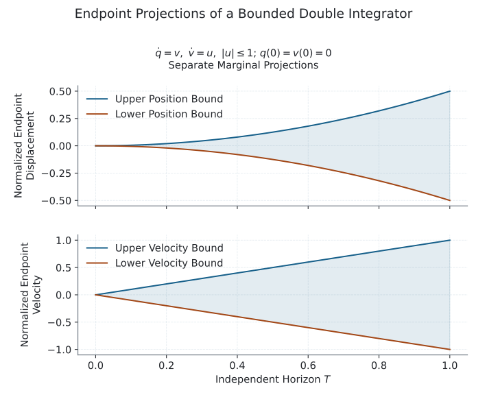
Long Description
For the declared normalized system \(\dot q=v\), \(\dot v=u\), \(|u|\leq1\), start every horizon \(T\in[0,1]\) from the same fixed initial state \(q(0)=v(0)=0\), with no state or input-rate constraints. The attainable endpoint position interval is \([-T^2/2,T^2/2]\) and the velocity interval is \([-T,T]\). Constant controls \(u=\pm1\) attain the respective extremes. These are exact marginal projections, not a claim that every position-velocity pair in their enclosing rectangle is jointly reachable. Acceleration drift is zero and acceleration-space DCR remains zero, although the full-state drift is \((v,0)\). The panels show how horizon changes attainable corrections in this model; they are not statistical dispersion, golfer delivery windows or calibrated time-to-impact bounds.7.1 Accessibility, Actuation and Gramians
An acceleration input acts immediately on velocity and subsequently on position. This distinction explains why full mechanical actuation does not mean the state input matrix has full row rank. In the scalar double integrator,
\[ \dot x=Ax+Bu,\qquad x=(q,v),\qquad A=\begin{bmatrix}0&1\\0&0\end{bmatrix},\quad B=\begin{bmatrix}0\\1\end{bmatrix}, \]
\(B\) has rank one, while \([B\;AB]\) has rank two. The acceleration drift is zero, so DCR is zero for a positive input capacity, but that fact alone does not describe how far position and velocity can change in a short time. With \(|u|\leq u_{\max}\), deviations from the unforced endpoint obey
\[ \delta v(T)=\int_0^T u(s)\,ds,\qquad \delta q(T)=\int_0^T(T-s)u(s)\,ds, \]
\[ |\delta v(T)|\leq u_{\max}T,\qquad |\delta q(T)|\leq\tfrac12u_{\max}T^2. \]
These are marginal bounds, not a claim that every pair in the enclosing rectangle is jointly attainable. They show why remaining time matters even when the drift ratio does not change.
For a trajectory-linearized perturbation model \(\delta\dot x=A(t)\delta x+B(t)\delta u\), let \(\Phi(T,s)\) be the state-transition matrix and \(R(s)\) a positive-definite input-cost metric. The weighted controllability Gramian is
\[ W_c(T)=\int_0^T\Phi(T,s)B(s)R(s)^{-1}B(s)^T\Phi(T,s)^T\,ds. \]
For the double integrator with \(R=1\),
\[ W_c(T)=\begin{bmatrix}T^3/3&T^2/2\\T^2/2&T\end{bmatrix},\qquad \det W_c=T^4/12>0\quad(T>0). \]
The Gramian describes the endpoint map under an integrated quadratic input budget. Its ellipsoids are not automatically the reachable sets for pointwise torque, rate or contact constraints. Eigenvalues also depend on state scaling and the input metric. Lie-bracket accessibility tests address another question, under their own hypotheses; neither input-map rank nor a scalar drift norm substitutes for those tests. In particular, multiplying a drift field by a large constant does not generally reduce accessibility rank.
7.2 Event-Level Path and Face Tests
Path and face are coupled outputs of a spatial golfer-club model. The planar chain can illustrate one projected motion, but it omits forearm axial rotation, much of wrist motion and spatial shaft deformation. It cannot establish preserved face authority, universal face error or a three-dimensional reachable-set shape.
A suitable comparison would start from the same state and admissible controls, propagate through a declared impact event, and report changes in clubhead velocity direction, face orientation and arrival time. It would vary inertial parameters, activation, shaft properties and impedance assumptions within declared uncertainty. A small correction should be compared with the required delivery tolerance; a quoted closure rate or isolated axial inertia does not supply that comparison.
8 Bounded DCR Validation Protocol
This protocol asks a narrower question than whether DCR is an appealing description: does a declared DCR add held-out information about a declared correction task beyond the state already known to the analysis? The analytic counterexamples come first. A positive association or prediction result cannot override a counterexample to a universal or theorem-level claim.
The current executable cases are analytic or deterministic synthetic systems. Parameter bounds are assumed inputs to those systems. No participant or golfer data are measured or estimated, and golfer task outcomes remain unavailable. This exploratory output is not coaching, clinical, design, causal, or population authority.
8.1 Protocol Declaration
Every run fails closed unless it records all of the following fields before results are examined:
| Required Field | Declaration |
|---|---|
| State and coordinates | Named initial-state values, coordinate frame or chart, and units. |
| Input set and bounds | Named admissible inputs, lower and upper bounds, units, and whether bounds vary with state. |
| Scaling and norm | Coordinate scaling or weighting and the exact norm used for DCR and task projections. |
| Finite horizon | Start state or phase, terminal time or stopping rule, and units. |
| Event definition | Guard surface, crossing direction, reset/contact rule, and event-time convention. |
| Task metric | Quantity being corrected, tolerance, and whether error is evaluated at fixed time or at the event. |
| Uncertainty model | Declared parameter/model set or probability model; unavailable uncertainty is reported as unavailable. |
| Solver and tolerance | Engine, solver and revision, step or analytic method, convergence test, and numerical tolerance. |
The executable ReachabilityProtocol binds those declarations. The scalar and planar system regressions extend src/affine_control/reachability.py; the zero-gradient and rank-deficient cases call the protected #4013 constant_additive_drift_interval API rather than defining a competing reachability calculation. Protocol and hypothesis records live in the separate orchestration layer src/affine_control/reachability_protocol.py.
8.2 Analytic and Deterministic Regression Matrix
The regression suite fixes six systems before any positive interpretation:
| System | Frozen Regression | What It Can and Cannot Establish |
|---|---|---|
| constant additive drift | With \(x_0=0\), \(\bar u=1\), and \(T=1\), drift 0 and 100 give \([-1,1]\) and \([99,101]\); both widths are 2. | Drift can translate a reachable set without shrinking it. This refutes universal scalar sufficiency, not a golf-specific effect. |
| state-dependent drift | \(\dot x=1+u\) and \(\dot x=x+u\), both at \(x_0=1\) with instantaneous DCR 1, have widths 2 and \(2(e-1)\approx3.4366\). | Equal instantaneous DCR does not fix finite-horizon width. |
| rank-deficient input map | For \(G=[1,0]^\mathsf{T}\), drift \((0,10)\), \(\bar u=1\), and \(T=1\), the box is \([-1,1]\times\{10\}\), input-map rank is 1, and area is 0. | A norm ratio does not encode directional rank or controllability. |
| saturation | A requested scalar correction of 2 with gain 1 and input bound 0.5 applies 0.5 and preserves an unmet residual of 1.5. | Constrained optimal correction depends on the task request and bounds, not DCR alone. |
| contact and event timing | Two height-1 cases with velocities \(-1\) and \(-3\), drift acceleration \(-9\), and control acceleration \(+1\) reach the event at about 0.3904 and 0.25. Event-velocity sensitivities to control acceleration are about 0.2425 and 0.2. | The same drift/control magnitude comparison can accompany different event maps because baseline state and speed differ. |
| model and parameter perturbations | For \(\dot x=ax+u\), \(x_0=1\), \(\bar u=1\), \(T=1\), and \(a\in\{0.8,1.0,1.2\}\), center spans \([2.2255,3.3201]\) and width spans \([3.0639,3.8669]\). | Assumed parameter variation is published as an envelope rather than hidden behind one ratio. |
All values above are analytic or modeled quantities from declared synthetic systems. They are not measurements. The exact numeric checks are in tests/test_dcr_event_sensitivity_protocol.py; a failed event, invalid bound, missing field, or nonfinite value is an explicit failure state rather than a substituted result.
8.3 Predeclared Hypotheses and Promotion Gates
- Association hypothesis: Test whether DCR remains associated with the declared task error after adjustment for baseline state, speed, and control authority. Report the coefficient, uncertainty interval, dependence structure, and missingness rule. Association does not imply intervention effect.
- Prediction hypothesis: Test whether adding DCR to that baseline reduces held-out task-error RMSE by at least a predeclared margin. Use group- or participant-held-out folds for participant data; the deterministic fixture uses leave-one-out cross-validation only to regression-test the calculation.
- Theorem-level hypothesis: Test any claim that scalar DCR alone determines correction authority against the complete counterexample matrix. One valid counterexample rejects the universal claim even if association or prediction is positive in a narrower dataset.
The current baseline-exact synthetic fixture gives both baseline and DCR-augmented held-out RMSE below the declared \(10^{-10}\) tolerance. Its incremental-prediction outcome is therefore null, not positive. The theorem-level scalar-sufficiency hypothesis is negative because the analytic counterexamples refute it. Association in golfers is unavailable because no participant data enter this protocol. Null and negative results remain in the ledger alongside supported and unavailable results; they are not filtered from publication.
For future measured data, preprocessing, folds, thresholds, model revisions, and hypothesis tiers must be frozen before inspecting outcomes. Cross-validation must compare the baseline state, speed, and control authority model with the same model plus DCR. Uncertainty must cover held-out error and declared parameter/model perturbations. A result can be promoted only within that dataset, model, event, task metric, and uncertainty envelope.
9 Stability and Clubface Variance: Required Model
A local perturbation analysis can begin with \(\delta\dot x=A(t)\delta x+B(t)\delta u\). It still needs a feedback policy, disturbances, measurement noise, initial uncertainty and an output map. For a local representation of face orientation \(\phi=h(x,t)\), \(\delta\phi=h_x\delta x\) describes a fixed-time state perturbation when there is no explicit time perturbation. It does not yet describe an impact-event output.
Let a smooth pre-impact trajectory cross the event surface \(g(x,t)=0\) at \(t_*\). If the crossing is transverse,
\[ g_t+g_x f^-\neq0, \]
where \(f^-\) is the complete pre-event velocity field, including the nominal input. With a small state perturbation \(\delta x^-\) evaluated at the nominal event time and a fixed event definition, first-order expansion gives
\[ \delta t_*=-\frac{g_x\delta x^-}{g_t+g_x f^-}, \]
\[ \delta h_*=h_x\delta x^-+(h_t+h_xf^-)\delta t_*. \]
All derivatives are evaluated on the nominal pre-event trajectory. Parameter changes in \(g\) or \(h\) add their own direct terms. A post-impact output additionally requires the reset/contact-map derivative and its timing convention. Near a grazing event the denominator can be small; the event sensitivity becomes ill-conditioned and the local approximation may fail. A trial that misses the event cannot be assigned a fabricated impact output.
For a check independent of golf assumptions, take height \(y_0=1\), initial vertical velocity \(v_0=-1\) and constant acceleration \(a=-8\) in consistent units. At the downward crossing of \(y=0\),
\[ v_*=-\sqrt{v_0^2-2ay_0}=-\sqrt{17},\qquad \frac{\partial v_*}{\partial a}=\frac{y_0}{\sqrt{v_0^2-2ay_0}}=\frac1{\sqrt{17}}. \]
This includes the changed event time. Holding the nominal time fixed instead would give \(\partial v(t_*)/\partial a=t_*\approx0.3904\), rather than the event derivative \(0.2425\). This difference is precisely why a same-time comparison and an impact comparison must not be interchanged.
If the resulting event-output Jacobian is \(J_e\) and the relevant small perturbations have covariance \(\Sigma\), a first-order covariance approximation is \(J_e\Sigma J_e^T\). Include the dependence between state, input and parameter errors when forming that covariance; do not add correlated uncertainties as if independent. DCR contains neither this map nor the covariance. A large drift magnitude does not imply a large state Jacobian or exponential error growth. The previous claim that path drift enforces face error remains withdrawn pending an event-level uncertainty study.
10 A Mechanical Counterexample to Monotone Growth
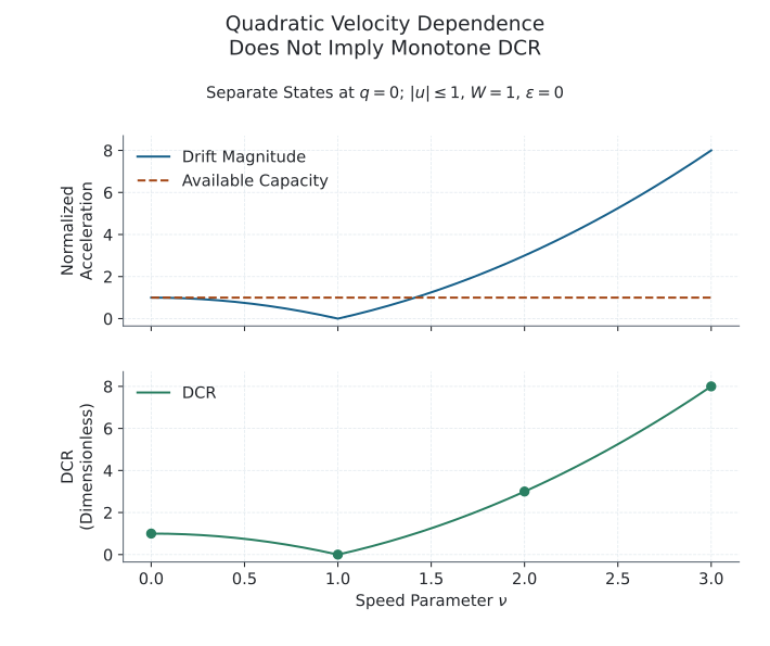
Long Description
The manufactured model derived below has \(\ddot q=1-\dot q^2+e^{-2q}u\). At separate states with \(q=0\), \(|u|\leq1\), \(W=1\) and \(\varepsilon=0\), drift magnitude is \(|1-\nu^2|\) and available acceleration capacity is one. The upper panel shows those acceleration quantities; the lower panel shows their dimensionless ratio, DCR. At speeds \(\nu=0,1,2,3\), DCR takes values \(1,0,3,8\). Cancellation first reduces drift magnitude to zero; increasing the speed parameter further makes it rise. The horizontal coordinate is a speed parameter, not elapsed downswing time. These states do not describe a trajectory that holds configuration fixed while velocity is nonzero, and the plot contains no golfer measurements or physiological capacity estimate.The curves in Figure 3 follow the declared mechanical example below, whose equations can be checked exactly. This is a manufactured model and a family of states, not a golfer trajectory or a downswing measurement.
Use dimensionless coordinate \(q\) and time \(s\), obtained after selecting reference coordinate, time and energy scales. Dots in this example refer to \(s\). Define normalized inertia \(I(q)=e^{2q}\), kinetic energy \(T=\tfrac12 I(q)\dot q^2\) and potential \(U=-\tfrac12e^{2q}\). The generalized input \(u\) is normalized consistently with those scales. Euler–Lagrange gives
\[ e^{2q}\ddot q+e^{2q}\dot q^2-e^{2q}=u, \qquad \ddot q=1-\dot q^2+e^{-2q}u. \]
The positive inertia makes this a valid local scalar Lagrangian model. The chosen potential is a mathematical construction, not a claim about gravitational geometry in a golfer. At the fixed configuration \(q=0\), with \(|u|\leq1\), a scalar absolute-value metric and \(\varepsilon=0\), the available acceleration capacity is one. Writing \(\nu=\dot q\),
\[ \mathrm{DCR}=|1-\nu^2|. \]
It takes values \(1,0,3,8\) at speeds \(\nu=0,1,2,3\). The velocity-dependent term is quadratic, yet drift magnitude first falls to zero through cancellation and then rises. If the realized input is fixed at \(u=0.2\), DIR is \(5|1-\nu^2|\). That larger ratio reflects the unused capacity in this declared policy, not a loss of available actuation.
| Speed \(\nu\) | Signed Drift | Available Capacity | DCR | DIR for \(u=0.2\) |
|---|---|---|---|---|
| 0 | 1 | 1 | 1 | 5 |
| 1 | 0 | 1 | 0 | 0 |
| 2 | \(-3\) | 1 | 3 | 15 |
| 3 | \(-8\) | 1 | 8 | 40 |
Each row is a separate state at the same configuration. It is not possible to traverse these rows as a continuous motion while keeping \(q=0\) and having nonzero \(\dot q\). The table isolates speed dependence intentionally. The symbolic derivation, metric comparisons, coordinate examples, Gramian and event derivative are checked independently in tests/test_dcr_article_rigor.py; the six governed cases above retain their separate executable evidence.
11 Limitations of This Analysis
The three-link geometry supplies a transparent model structure. It supplies no calibrated golfer parameter set, measured input history or validated finite-horizon golf result. Its planar rigid-link assumptions omit spatial coordination, activation dynamics, tendon and shaft states, and contact changes unless those are explicitly added. Adding them can change the state, input map, baseline and admissible controls, rather than merely adjusting a single inertia number.
No universal physiological torque envelope is assumed. Ideal bounded inputs in the exact examples are declared mathematical inputs. Estimating an individual’s capacity requires measurements and a muscle/joint model; observed motion alone does not separate all internal forces or identify unused capacity. An inverse-dynamics net torque is not automatically a muscle activation or a signal-dependent noise level.
The local derivatives and linearizations apply to small perturbations within their assumptions. They do not certify global correction, stability through contact, or uncertainty coverage for an unmeasured golfer. The deterministic counterexamples establish limits on universal reasoning. They leave open whether a carefully specified DCR adds useful predictive information in a particular measured dataset.
12 How the Mechanisms Connect
Preparation changes configuration, velocity, activation and elastic state. Those states determine the subsequent drift and the input map in a chosen model. Activation and geometry also help determine admissible force; remaining time and directional coupling determine how that force can change club delivery. Contact then determines when and how the delivery outcome is evaluated. Measurement uncertainty affects each step.
This chain gives DCR a useful, bounded place: report a local acceleration comparison while retaining the underlying state, metric and input bounds. Use forward interventions for questions about removing or holding an input, energy balances for questions about storage and transfer, and event-level reachable or sensitivity calculations for questions about correction. A large ratio does not answer all three.
For example, early activation can prepare impedance and tendon strain that affect a late perturbation response. Calling that response part of a held baseline does not make its physiological preparation irrelevant. Similarly, shaft deformation can affect the face and path together without establishing that flexibility improves a player’s result. These connections motivate testable comparisons between complete models and measured outcomes.
13 Primary Sources and Reproduction
The MIT multibody dynamics notes provide the Lagrangian and manipulator-equation foundation used here. They are mathematical course notes, not evidence for a golf-specific DCR trajectory. The original Harris and Wolpert paper introduces the signal-dependent-noise hypothesis discussed above; its eye and arm modeling does not validate a golfer DCR claim.
The worked mathematical examples are derived in this article with explicit assumptions and independently checked in the repository tests. The bounded protocol retains analytic, null, negative and unavailable outcomes. The previous video descriptions and timestamps have been removed because they were not verified as supporting the claims attributed to them. A general dynamics or relativity resource cannot serve as evidence for a golf-swing correction limit.
14 Acknowledgments
Computational modeling assistance and structured drafting support for this article were provided by ChatGPT (OpenAI). All theoretical content, arguments, and conclusions are the work of the named author.
Citation
@online{olson,
  author = {Olson, Dieter},
  title = {Drift, {Control} {Capacity} and {Golf-Swing} {Correction}},
  url = {https://affinedrift.com/articles/drift-control-ratio.html},
  langid = {en}
}