Zero-Torque Counterfactual (ZTCF) Family
Plain-Language Summary
This article explains the Zero-Torque test step by step. The method shows what the club does when muscle push stops, without guessing what the golfer intended.
Key Takeaways
- ZTCF computes the forward-dynamics trajectory that results when muscular torques are set to zero.
- The counterfactual isolates passive drift evolution under identical initial phase conditions.
- Does not claim human golfers can physically execute an identical swing without muscle activation.
These entries remain visible until evidence-backed adjudication changes their governed status.
- Open / Medium: Critique: Passive Overshoot Artifact (Simulink "Proof") (
crit-passive-overshoot-artifact) - Open / Medium: Critique: The Static Fallacy (Zero Velocity Counterfactual) (
crit-static-fallacy-zvcf) - Open / High: Critique: Identifiability and "Input" as a Residual (
crit-ztcf-identifiability)
New to control theory? Here is what the Zero-Torque Counterfactual means in everyday language.
The Model Branch
Freeze the modeled swing at the top of the downswing. Where would the club go if the model's declared applied control were zero here? This is a forward Zero-Torque Counterfactual (ZTCF). Only what the record keeps remains: forces, constraints, contacts and internal states.
Why Does This Matter?
Comparing two model branches gives a simulated path difference. Reading it as a contribution or a cause needs extra assumptions. It does not identify muscle forces, co-contraction, effort or intent.
A Thought Experiment, Not a Real Swing
Zero here means zero in the declared applied-control channel under the stated model. It is not a measurement of muscle state. A generalized torque can be zero under one coordinate choice while muscle forces, co-contraction or contact loads stay nonzero and unidentified. Stiffness and damping stay only if the record declares them as fixed parameters or internal states. The intervention does not show they were identified from a golfer or can be held apart from activation.
- Established (textbook): Lagrangian drift/input decomposition of control-affine systems; counterfactual simulation as a diagnostic technique in mechanics.
- Project convention: Applying the ZTCF family to declared golf models and requiring a machine-readable intervention record before publishing a result.
- Terminology: “Zero Torque Counterfactual (ZTCF)” is the authors’ label for this construction in the golf context; the underlying mathematics is standard rigid-body dynamics.
This article is the canonical reference for “ZTCF” across the AffineDrift site. All other articles should link here on first use. Four related objects are in circulation; the qualifier is required on first use:
Pointwise ZTCF sample — \(f(x(t))\), the zero-applied-control evaluation at one achieved state. It is an instantaneous vector, not a forecast. “Pointwise drift vector” is the preferred generic name; “pointwise ZTCF sample” is retained for compatibility with the WSCG archive and must carry the qualifier.
Stitched pointwise ZTCF trace — the time-indexed collection \(\{f(x(t_k))\}\) evaluated along achieved states. Its samples do not form a dynamically integrated trajectory because each sample is reset to a different achieved state. It supports same-state attribution but cannot establish persistence after control removal.
Forward ZTCF trajectory — \(x^{\mathrm{ZTCF}}(t; x_0, t_0)\), the solution of \[\dot{x}^{\mathrm{ZTCF}}(t) = f\!\left(x^{\mathrm{ZTCF}}(t)\right), \qquad x^{\mathrm{ZTCF}}(t_0) = x_0, \qquad t \in [t_0, t_1].\] This is a dynamically integrated trajectory, not a pointwise sample.
Branched ZTCF trajectory — the forward ZTCF trajectory (3) initialized from an achieved or simulated reference state \(x_0 = x^{\mathrm{reference}}(t_0)\), then compared with a separately integrated reference branch for \(t > t_0\). A publishable result requires the intervention record below; the construction name alone is not validation.
The drift vector field \(f:\mathcal{X}\rightarrow T\mathcal{X}\) is the state-dependent map underlying all four constructions. It is not a trajectory or a dataset. Pointwise and stitched results may support same-state attribution; only a forward or branched rollout can test whether an effect persists after the applied control is removed.
Articles must qualify the construction on first use and either link to this definition or state the local convention explicitly.
1 Worked Example: Evaluating a Pointwise Sample
Given: the default three-link GolfModel() (masses \((10,5,0.81)\) kg, lengths \((0.3,0.35,1.15)\) m) at rest, \(q=(0,0,0)\), \(\dot q=(0,0,0)\).
Steps:
- Call
GolfModel().drift_acceleration(q, qd)withq = qd = (0, 0, 0). - This solves \(M(q)\ddot q=-h(q,\dot q)\) for the bias load \(h\) (gravity plus Coriolis), giving the pointwise sample \(f(x(t_b))\) from item 1 above.
Result: \(f(x)\approx(-31.40,\ 29.98,\ 1.57)\) rad/s\(^2\) — one pointwise sample at one achieved state. It is not integrated forward and does not by itself predict the freely evolving forward ZTCF trajectory of item 3 above.
Computed by src/affine_control/golf_model.py::GolfModel.drift_acceleration; checked against this page by tests/test_worked_example_callouts.py::test_ztcf_pointwise_sample_at_rest.
2 Normative Intervention and Interpretation Contract
Every executable or quantitative ZTCF result must conform to affinedrift.ztcf-intervention/v1. The normative schema and golden fixture make the following fields reviewable:
| Contract Area | Required Declaration |
|---|---|
| Model authority | Model ID and version, exact source revision, engine and engine version, and all parameters needed for replay |
| Branch state | Coordinates, values, units, reference frame, and the provenance of the initial state |
| Intervention | Physical level and exact channels set to zero; no implication that another torque, activation, or force was removed |
| Retained inventory | Other controls, constraints, contacts, external loads, internal states, and parameter-freezing rule |
| Integration | Start and end time, units, solver and version, steps or tolerances, and finite-horizon postconditions |
| Interpretation | Simulated trajectory difference, contribution measure, causal estimand, physiological interpretation, and non-identifiability limits as separate fields |
| Failure | invalid_contract, engine-unavailable, engine-unsupported, and numerical_failure are fail-closed states, not missing values that another result may fill |
The registered fixture supports only the repository’s Python GolfModel.ztcf_trajectory/v2 algorithm for one declared planar model. It is a deterministic software regression, not a human or cross-engine validation. MATLAB, Simulink, MuJoCo, Pinocchio, and other engines have no parity claim under this contract unless a second supported adapter, exact model translation, golden fixture, metric, and tolerance are registered.
The current fixture uses model version 2.0: a rigid three-link chain with consistent rigid inertia and bias forces. It integrates no flexible shaft states or additional shaft inertia. The historical version 1 fixture is preserved as a record of the earlier mixed-inertia calculation and is unsupported by the current adapter. The model change requires a new result; it does not inherit the old numerical or physical interpretation.
2.1 Interpretation Ladder
These outputs must not be collapsed into one claim:
- A simulated trajectory difference compares two numerical branches.
- A contribution measure adds a declared projection, norm, event, or work functional.
- A causal estimand additionally requires a defensible intervention, exchangeability or structural assumptions, and treatment of model discrepancy.
- A physiological interpretation requires measurements and an identifiable mapping from generalized inputs to muscle, tissue, neural, or effort quantities.
The first item does not imply the next three. Each result must state its non-identifiability boundary even when numerical replay succeeds.
3 Motivation
Golf-swing models combine inertial, gravitational, elastic, damping, contact, and declared input terms. Inverse dynamics estimates net generalized quantities under a model and measurement pipeline; it does not uniquely allocate them to individual muscles, tissues, co-contraction, or intent.
The drift–input decomposition of the control-affine system \(\dot{x} = f(x) + G(x)u\) provides the formal separation between passive dynamics \(f(x)\) and input-driven dynamics \(G(x)u\). However, this separation is instantaneous: it classifies the current velocity of the state, not the trajectory over time. The state reflects earlier inputs and loads. A forward calculation asks how that state evolves under a newly specified input protocol; it does not recover a unique history from the current state.
To convert the instantaneous decomposition into a trajectory-level diagnostic, we integrate the drift-only equations forward from a chosen initial state. The resulting trajectory is the forward Zero-Torque Counterfactual (ZTCF) trajectory.
4 Formal Definition
4.1 Control-Affine Setting
For a declared model and constraint/contact mode whose complete state equations are affine in the selected generalized-torque input, write:
\[\dot{x} = f(x) + G(x)\,u, \qquad x(t_0) = x_0,\]
where:
- \(x=(q,v,z)\) is the complete declared state: coordinates, velocities and any internal states such as flexible modes, actuator states or controller memory; the registered rigid fixture uses only \((q,v)\),
- \(f(x)\) is the full-state derivative with the selected applied input zero; its mechanical acceleration block is distinct from its coordinate and internal-state derivatives,
- \(G(x)\) is the input matrix — how applied joint torques enter the equations,
- \(u(t)\) is the declared vector of applied generalized torques, not an identified vector of muscle forces or activations,
- \(t_0\) is the initial time at which the counterfactual branches.
The autonomous notation used here assumes that retained loads and policies have no explicit time dependence, or that the required clock/controller states have been included. Otherwise use \(f(x,t)\) and \(G(x,t)\) and retain the prescribed time-dependent protocol. Zeroing selected channels while leaving a controller active does not make the remaining plant autonomous. A recorded input replay and a feedback policy reacting to the changed state are different reference protocols.
The drift field \(f\) contains exactly the effects assigned to it by the declared effective plant. Depending on the record, those may include inertial coupling, Coriolis and centrifugal terms, gravity, elastic or damping forces, contact, and exogenous loads. Calling the field passive does not make its inventory universal or physiologically identified.
4.2 The ZTCF Trajectory
Let \(x(t)\) denote the reference trajectory of the declared model under a specified torque input \(u(t)\) on the interval \(t \in [t_0, t_f]\), with initial condition \(x(t_0) = x_0\).
We define the forward Zero-Torque Counterfactual trajectory, denoted \(x^{\mathrm{ZTCF}}(t)\), as a solution of the declared drift-only initial value problem:
\[\boxed{\dot{x}^{\mathrm{ZTCF}}(t) = f\!\left(x^{\mathrm{ZTCF}}(t)\right), \qquad x^{\mathrm{ZTCF}}(t_0) = x_0.}\]
By construction:
- The branch state, coordinates, units, and frame are recorded explicitly.
- Parameters, constraints, contacts, loads, and internal states follow the retained-inventory record.
- The named generalized-torque channels are held at zero over the declared finite horizon.
Existence and uniqueness require the usual initial-value regularity over the declared horizon. A singular constraint solve, undefined contact transition, nonfinite state, unavailable engine, or unsupported algorithm is a failure state; it is not replaced by an inferred trajectory.
4.3 The Torque-Driven Deviation
Along the reference trajectory, the state derivative contains both drift and input contributions:
\[\dot{x}(t) = f\!\left(x(t)\right) + G\!\left(x(t)\right)\,u(t).\]
Along the ZTCF trajectory, the derivative contains only the drift:
\[\dot{x}^{\mathrm{ZTCF}}(t) = f\!\left(x^{\mathrm{ZTCF}}(t)\right).\]
Within the fixed declared plant, setting \(u=0\) removes the term \(G(x)u\). The two branches then visit different states, so their difference is a model-conditioned simulated trajectory difference. It is not automatically an additive torque contribution, a causal estimand for a real golfer, or a physiological interpretation.
5 Geometric Interpretation
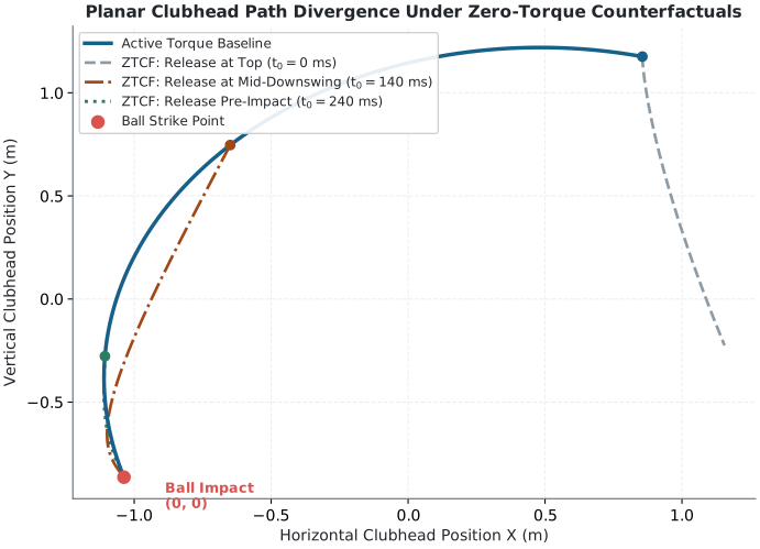
Long description
The trajectory plot compares the spatial paths traced by the clubhead in the swing plane. The nominal trajectory with continuous muscular torque curves smoothly into impact. Counterfactual paths branched at earlier milestones diverge markedly: zero torque from the top of the downswing yields a wide, flailing arc that fails to square the club, while branching at mid-downswing preserves initial momentum but suffers significant path deviation. Branching in the final 30 ms before impact follows the nominal path closely, showing that passive kinetic momentum dominates the terminal geometry.When the initial-value problem is well posed, a forward ZTCF is an integral curve of the declared drift vector field \(f\) through \(x_0\) at time \(t_0\).
A model may retain the following effects when its record declares them; this list is broader than the registered rigid fixture:
- Inertia and momentum — the mass distribution defines the inertia matrix; together with the current generalized velocity it determines generalized momentum \(p=M(q)v\) in the stated rigid-coordinate model,
- Centrifugal and Coriolis forces — arising from the high-speed rotation of the arm-club chain,
- Elastic shaft recoil — the restoring force of the bent shaft as it tries to return to its neutral shape,
- Passive joint damping — any modeled energy dissipation in the joints.
What is absent from the forward ZTCF is the declared applied generalized-control input. Passive tissue, joint, shaft, contact, damping, and structural forces remain if they are included in \(f\). The difference between \(x(t)\) and \(x^{\mathrm{ZTCF}}(t)\) captures the cumulative modeled consequence of removing that input; it does not uniquely recover muscle forces. Broadly:
- Close branches show a small difference in the declared metric and horizon; they do not prove that control, muscle activity, or effort was small.
- Within an exact fixed deterministic model, the paired difference follows from the specified intervention and retained protocols. Comparing a computed branch with human data additionally introduces state-estimation error, parameter uncertainty, omitted loads, contact mismatch and model discrepancy. Numerical error affects either comparison.
6 Relationship to the Drift–Input Decomposition
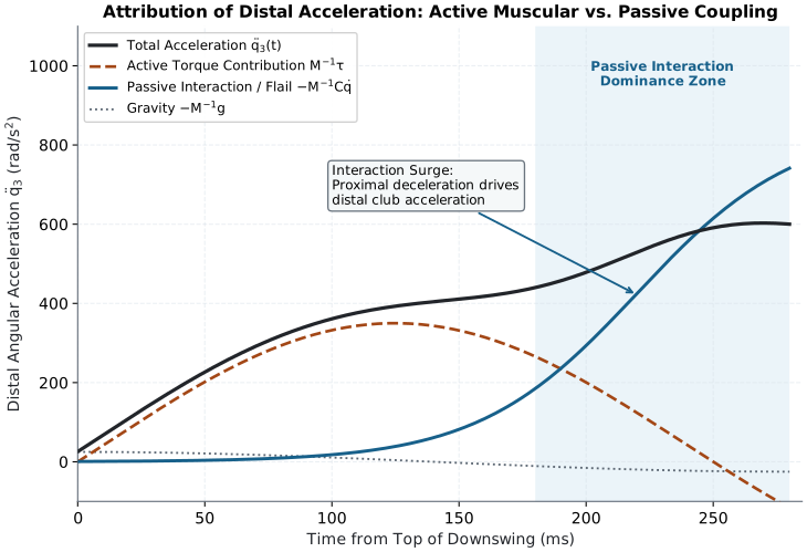
Long description
The acceleration decomposition graph displays the relative contributions of torque and passive dynamics to distal angular acceleration over the downswing duration. In the early transition phase, active muscular torque \(M^{-1}\tau\) provides virtually all acceleration. Passing the halfway point, velocity-dependent Coriolis and centrifugal terms \(-M^{-1}C\dot{q}\) surge, rapidly eclipsing muscular input. Near impact, interaction forces drive the majority of clubhead acceleration, illustrating the whip-like energy transfer characteristic of double-pendulum dynamics.The drift–input decomposition used throughout this series is the algebraic identity:
\[\dot{x} = \underbrace{f(x)}_{\text{declared drift}} + \underbrace{G(x)\,u}_{\text{applied input}}.\]
This identity is instantaneous: it classifies the current velocity vector at a single point in time. A forward ZTCF extends the instantaneous evaluation into the temporal domain by integrating the declared drift field.
6.1 Generalized Load Is Not an Inverse-Dynamics Input
For an unconstrained fully actuated rigid model, use one sign convention:
\[M(q)a+h(q,v,z)=u,\qquad a_0=-M^{-1}h.\]
Define the inertial generalized load as \(Q_{\mathrm{inertial}}=Ma\) and the retained generalized load as \(Q_{\mathrm{retained}}=-h\). Then
\[u=Q_{\mathrm{inertial}}-Q_{\mathrm{retained}}=M(a-a_0).\]
A hypothetical scalar component of \(Ma\) equal to \(100\) N·m and the corresponding retained load equal to \(85\) N·m leaves an applied input of \(15\) N·m. If inverse dynamics already reports the required input as \(100\) N·m, subtracting \(85\) again double counts the retained dynamics. The same model can compute all these quantities. A signed component ratio is not a muscle-effort fraction and can change with coordinates or cancellation between terms.
With an input map \(B\), the same-state acceleration difference identifies \(Bu=M(a-a_0)\), which may not identify a unique input. With constraints, use the full acceleration/reaction solve. The paired textbook chapter derives a two-rod example from COM kinetic energy and shows why dropping off-diagonal mass terms produces the wrong recovered input.
6.2 Constraints and Output Acceleration
At a fixed feasible equality-constraint mode, solve
\[ \begin{bmatrix}M&-A^T\\A&0\end{bmatrix} \begin{bmatrix}a\\\lambda\end{bmatrix} =\begin{bmatrix}Bu-h\\b\end{bmatrix}. \]
Here \(Aa=b\) includes constraint curvature and prescribed support motion. Positive-definite \(M\) and independent constraint rows make the equality solve well posed. The zero-input baseline contains reactions and is generally not \(-M^{-1}h\). Unilateral contact and friction conditions must remain feasible; a branch may require a different contact mode or an explicitly modeled impact.
For a fixed geometric point \(y(q)\), acceleration is \(Ja+\dot Jv\). At a common state the input increment is \(JHu\), where \(H\) is the constrained input-to-acceleration operator. On separated branches the Jacobian and transport term can differ. Joint acceleration, clubhead acceleration, speed change and energy flow are different outputs.
7 Relationship to DCR and Reachability
DCR compares declared drift and bounded input-effect magnitudes in one projection and metric. It does not establish that a forward ZTCF approaches an achieved trajectory, that the ZTCF is an attractor, or that other finite-horizon outcomes are unreachable. Those questions require the admissible control set, horizon, task metric, uncertainty, and event definition documented in the corrected Drift-Control Ratio article. A ZTCF branch remains one model-conditioned intervention at every DCR value.
8 Numerical Algorithm
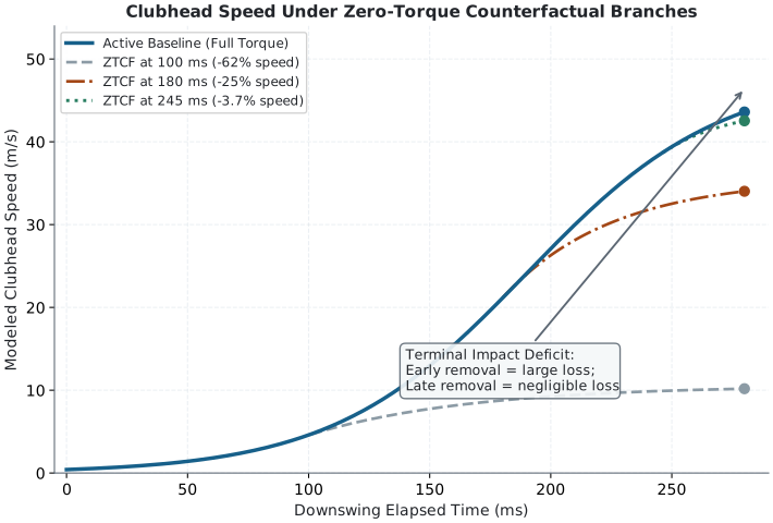
Long description
The velocity profile comparison illustrates clubhead speed development from takeaway to impact. The active swing achieves a peak velocity of approximately 48 m/s at contact. If torque is removed at transition, the clubhead reaches less than 20 m/s. Branching at mid-downswing caps speed at 35 m/s. However, releasing torque within 30 ms of impact results in negligible speed reduction, quantitatively proving that late muscular forcing contributes minimally to terminal kinetic energy compared to the passive flail mechanism.This section describes the generic integration pattern. The only governed executable result published here is the Python golden fixture linked in Section 2. No current MATLAB or Simulink model/version/input record or cross-engine parity artifact is registered, so results attributed to those engines are unavailable under this contract.
8.1 Notation and Discretization
Let the continuous-time state be
\[x(t) = (q(t),v(t),z(t)),\]
and let the simulation produce samples at discrete times
\[t_k = t_0 + k\,\Delta t, \qquad k = 0,\dots,N.\]
Let:
- \(x_k\) denote the simulated state at time \(t_k\),
- \(u_k\) denote the applied torque input at \(t_k\),
- \(f(x_k)\) denote the full-state drift derivative at \(x_k\), including its mechanical acceleration block,
- \(x^{\mathrm{ZTCF}}_k\) denote the ZTCF state at time \(t_k\).
8.2 Branch-Switch Pattern
A branch-switch implementation must capture the complete declared state, set only the registered input channels to zero, apply the retained contact/load/ constraint protocol, and integrate with the registered solver to the registered horizon. Describing a switch block is not evidence that an engine implements that contract. Engine-unavailable and engine-unsupported requests fail closed.
8.3 Discrete-Time Integration
For a general-purpose discrete implementation, the ZTCF trajectory can be approximated by integrating the drift field:
\[x^{\mathrm{ZTCF}}_{k+1} = x^{\mathrm{ZTCF}}_k + \Delta t\,f\!\left(x^{\mathrm{ZTCF}}_k\right) + \mathcal{O}(\Delta t^2),\]
with the initial condition \(x^{\mathrm{ZTCF}}_0 = x(t_0)\).
Euler has first-order global accuracy for a sufficiently smooth well-posed problem on a fixed interval; the displayed remainder is the one-step local error, not the accumulated error. Choose a method using stability, accuracy, events and convergence evidence. Large acceleration or nonlinearity alone does not establish stiffness. Rapidly decaying modes relative to the solution time scale can impose a restrictive explicit stability limit, as described in the SUNDIALS mathematical documentation. Contact discontinuities additionally need a declared event or nonsmooth treatment.
Numerical protocol requirements:
- Adaptive solvers may be used only with recorded implementation/version, tolerances, event behavior, and convergence evidence.
- Fixed-step solvers require their method, step count or size, endpoint rule, and refinement check.
8.4 Consistency Verification
At every common state, verify the affine acceleration identity using the full forward solve:
\[a(x,u,t)-a(x,0,t)=H(x,t)u.\]
The two branches start at a common state, but usually occupy different states afterward. Their acceleration difference then contains both the input effect and the changed baseline:
\[a(x^r,u,t)-a(x^0,0,t)=a_0(x^r,t)-a_0(x^0,t)+H(x^r,t)u.\]
An identity checked once does not establish correct integration. Also check forward/inverse closure, constraint residuals, appropriate energy or power balance, and step refinement of the stated output. A constant acceleration can be very large while its state Jacobian has only zero eigenvalues; that fact alone introduces no fast damped mode.
8.5 Zero-Velocity Evaluation Is a Different Intervention
For an unconstrained model, the instantaneous ZVCF slice is
\[a_{\mathrm{ZVCF}}(q,z,t)=-M(q)^{-1}h(q,0,z,t).\]
With identical remaining state, parameters and load protocol, define
\[a_{\mathrm{velocity}}=a_0(q,v,z,t)-a_{\mathrm{ZVCF}}(q,z,t).\]
The second subtraction isolates the effects changed by the specified velocity reset. It does not equal the difference between applied input and configuration-only drift. Gravity is the only surviving bias only in a model whose other retained loads vanish at zero velocity. Elastic strain, internal-state forces and prescribed loads can remain.
State which velocities are reset, including any stored in internal states, and check constraint feasibility before evaluating. A moving constraint \(q=t\) requires \(\dot q=1\) and does not permit zero velocity. A feasible reset changes kinetic energy and is distinct from removing an applied torque. Integrating after a reset creates a separate initial-state intervention; it is not the instantaneous ZVCF evaluation itself.
8.6 Practical Considerations
Consistent parameter sets. All inverse-dynamics evaluations and drift field computations must use the exact same inertia, stiffness, and damping parameters to ensure numerical consistency. In an unconstrained fully actuated model, the recovered input \(M(a-a_0)\) should match the directly applied input. For other input maps or constrained models, verify the complete generalized force and reaction balance.
Solver declaration. A comparison must declare both solvers, versions, tolerances or step sizes, endpoint behavior, and numerical sensitivity. Using the same solver can reduce one source of discrepancy but does not validate the model or intervention.
Measurement processing. Differentiation amplifies motion-measurement noise. Report reconstruction, filtering, differentiation, synchronization and uncertainty together; smoothing trades noise reduction against bias and bandwidth, and does not guarantee accurate accelerations.
Event definition. A fixed-time output differs from an output at each branch’s impact event. State event localization and what is reported if the branch never reaches impact. A missing event is not assigned the reference branch’s value.
9 Interactive Counterfactual Explorer
Pick an intervention time. The explorer integrates one declared, constant joint torque from the registered fixture state, then branches a zero-torque counterfactual from the actual state at that time and runs both to the same horizon.
Exploratory model output
— Declared-torque run · - - Zero-torque branch from ti · grey: the chain at ti. Thick lines show both chains at the horizon; thin lines trace the club tip.
Clubhead speed (m/s) against time, range —
| At the 0.2 s horizon | Value |
|---|---|
| Clubhead speed, declared-torque run (m/s) | — |
| Clubhead speed, zero-torque branch (m/s) | — |
| Simulated difference, run minus branch (m/s) | — |
| Joint-angle difference Δq1, Δq2, Δq3 (rad) | —, —, — |
Sampled clubhead speeds (data table)
| t (s) | Declared-torque run (m/s) | Zero-torque branch (m/s) |
|---|
Provenance. Model, parameters and initial state come from
data/ztcf/planar_golf_forward_fixture_v2.json, SHA-256
65c56f993d7e4eb2fb30efca1cd264f6eead8b2727e3fe010d8f1f885cccc021.
The declared torque is (40, 15, 3) N·m, held constant; it is illustrative and
not fitted to a golfer. The Python reference writes each branch as a
ZTCFIntervention record and replays it through
execute_ztcf_intervention; the browser mirror is checked against it by
tests/fixtures/widgets/ztcf-explorer.parity.json.
What the difference does not identify. No contribution fraction is identified, and generalized-torque removal does not identify muscle activation, force, effort, or intent. The fixture names these as not identified:
- individual muscle forces
- co-contraction and impedance cost
- unmodeled loads or contact changes
- human strategy or coaching outcome
Open critiques of this page: Identifiability and "Input" as a Residual (high), The Static Fallacy (Zero Velocity Counterfactual) (medium) and Passive Overshoot Artifact (medium).
This is an exploratory model output. Watch how the difference changes with \(t_i\). It need not shrink steadily as the intervention moves later, because each branch starts from a different state that the torque helped reach. The difference is a simulated trajectory difference inside this model; reading it as a share of speed “supplied by the golfer” needs the extra assumptions discussed in the critiques above.
9.1 The Same Branch, Animated
src/affine_control/ztcf_explorer.py, src/affine_control/golf_model.py, src/affine_control/ztcf_contract.py, data/ztcf/planar_golf_forward_fixture_v2.json. It does not play by itself.Transcript
A three-link model runs under a declared, constant joint torque.
At the intervention time, we copy the state of the model.
From that copy, a second branch runs with the torque set to zero.
Solid: the declared-torque run. Dashed: the zero-torque branch.
The gap at the end is a simulated difference inside this model.
It is not a share of speed supplied by the golfer, and not a muscle measurement.
10 Scope and Limitations
10.1 What the ZTCF Answers
The ZTCF answers a precisely defined question within the mechanical model:
“Under this exact model record and retained-inventory protocol, what branch is computed when these declared applied generalized-torque channels are set to zero from \(t_0\) to \(t_1\)?”
It does not claim that such a motion could be physically achieved by a real golfer, that the nervous system selects zero torque, or that the numerical branch isolates a unique biological cause. It is a model-conditioned intervention on named inputs.
10.2 Key Limitations
The ZTCF trajectory is not directly observable from real golf swing data. Three identifiability challenges apply:
Generalized torque is not muscle state. Net generalized torque, individual muscle forces, activation, co-contraction, impedance, and metabolic effort are different quantities. Zeroing one modeled torque vector identifies none of the others.
Requires a complete dynamic model. To evaluate \(f(x)\) at the measured state, one needs the declared mass matrix, complete bias forces, constraints, loads and any internal-state dynamics. Flexible-shaft parameters are needed only when that model includes flexibility; the registered rigid fixture does not. Each parameter introduces model uncertainty that propagates directly into the ZTCF estimate.
Initial condition and model sensitivity. A nonlinear rollout can amplify initial-state, parameter, contact, and solver differences. Reliability is case-specific; no universal short-horizon duration is asserted without a registered sensitivity result.
ZTCF software should first pass manufactured or golden-fixture checks, then model and measurement uncertainty must be evaluated separately. Passing a software fixture is not validation against real swing data.
This is not a no-muscle simulation. It is a declared generalized-input intervention whose physiological interpretation remains unavailable without an identified musculoskeletal model and supporting measurements.
10.3 Available Numerical Evidence
The registered Python golden fixture verifies deterministic replay of one 10-millisecond, three-link planar rollout against an exact model/version/input record. Cross-engine parity, spatial contact, time-varying impedance, human model adequacy, causal identification, and physiological validation are unavailable. A future result must add its own conforming intervention record rather than inheriting the fixture’s authority.
11 See Also
- The Physics of Golf: Chapter 6 Zero-Torque Counterfactual — Textbook derivation of ZTCF, DCR, and drift–input decomposition in golf mechanics
- Part 1: Control-Affine Framework — Derivation of \(\dot{x} = f(x) + G(x)u\) and the mechanical separability of drift and input
- Part 2: ZTCF and ZVCF Tools — Full treatment of both counterfactuals, including ZVCF definition and drift invariance discussion
- Part 5: Numerical Validation — Historical numerical discussion whose results require migration to the normative intervention contract
- Drift-Control Ratio — Boundaries between a scalar magnitude ratio and finite-horizon reachability
12 Revision History
2026-09-29: Extended critique annotations to ZTCF and proximal-distal pages (#4524).
2026-09-23: Corrected zero-torque mechanics and reconciled counterfactual reasoning (#4430).
2026-09-08: Standardized cross-article category metadata and link targets (#4302).
2026-08-20: Standardized and harmonized ZTCF, ZVCF, DCR, Drift, and Control definitions (#3889).
Citation
@online{olson,
  author = {Olson, Dieter},
  title = {Zero-Torque {Counterfactual} {(ZTCF)} {Family}},
  date = {},
  url = {https://affinedrift.com/articles/zero-torque-counterfactual.html},
  langid = {en},
  abstract = {This article presents the full mathematical and numerical
    formulation of the Zero-Torque Counterfactual (ZTCF) family. It
    describes integration algorithms, boundary intervention conventions,
    and causal attribution limits for isolating passive momentum
    transfer from active muscle torques in the golf swing.}
}