Theory Series, Part 4: Worked Pendulum Dynamics
Beam Reduction and Reproducible Pendulum Dynamics
Plain-Language Summary
This article works through the math of a swinging rod and bending shaft. It shows how shaft bend and wrist turns work together in a simple model.
Key Takeaways
- Explicit mechanical derivations link shaft bending and gravity to joint boundary reactions.
- Control input contributions can diverge in direction from total resultant accelerations.
- Multi-link pendulum approximations clarify kinetic energy transfer between proximal and distal segments.
These entries remain visible until evidence-backed adjudication changes their governed status.
- Open / High: Critique: Input-Dependent Boundary Conditions (The Grip Paradox) (
crit-input-dependent-boundary-conditions)
What These Examples Establish
These appendices derive the equations of declared mechanical models and provide reproducible numerical examples. They show how gravity, shaft bending, torque, and boundary conditions interact. They also show why an input contribution can point in a different direction from the total acceleration.
The calculations check internal consistency. Whether a model predicts a golfer’s motion or explains physiology requires suitable measurements and separate validation. A simpler model is useful when its assumptions and the question it can answer are explicit.
Appendix A: Consistent Coupled Dynamics
The purpose of these appendices is to make the mechanical calculation reproducible. An exact identity within a declared model does not prove that the model captures a golfer’s physiology, contact behavior, or variability. The independent examples below separate those questions.
Coordinates, Loads, and the Complete Mass Matrix
Use independent local coordinates \(z=(q,\eta)\), velocity \(v=\dot z\), and state ordering \(x=(q,\dot q,\eta,\dot\eta)\). The retained kinetic energy defines \(M(z)\) by \(T=\tfrac12v^\top Mv\). Assemble the rigid segments, shaft translation, and head translation and rotation using their actual placements and consistent reference frames, as developed in Part 1. For independent coordinates with positive kinetic energy in every nonzero velocity direction, \(M\succ0\). Redundant coordinates, ideal locks, singular charts, and changing constraints require an appropriate constrained formulation; adding an inverse symbol does not solve those cases.
Let \(g_z=\partial_z U_g\) include both rigid and modal gravity. Keep a declared passive joint load \(\tau_{\mathrm{pas}}\) in every equivalent form of the equations. With fixed modal stiffness and damping,
\[ M(z)\dot v+C(z,v)v+g_z(z) +\begin{bmatrix}\tau_{\mathrm{pas}}\\K_s\eta+C_s\dot\eta\end{bmatrix} =\begin{bmatrix}B(q)u\\0\end{bmatrix}. \tag{1}\]
The zero lower input block denotes absence of direct modal actuation. It does not eliminate modal loads or acceleration. The input matrix \(G(x)\) below is different from the gravity load \(g_z\). The blocks \(M_{rr},M_{rf},M_{fr},M_{ff}\) are respectively \(M_{qq},M_{q\eta},M_{\eta q},M_{\eta\eta}\); the rigid-coordinate block includes every body’s contribution when the retained modal rates are zero. For the standard Christoffel construction in coordinate velocities, \(\dot M-2C\) is skew-symmetric. Arbitrary velocity variables require their own kinematic and balance equations.
Define \(h=Cv+g_z+[\tau_{\mathrm{pas}};K_s\eta+C_s\dot\eta]\). Then
\[ M\dot v=-h+\begin{bmatrix}Bu\\0\end{bmatrix}. \tag{2}\]
Solving the same system gives
\[ \dot v=-M^{-1}h+M^{-1}\begin{bmatrix}B\\0\end{bmatrix}u. \tag{3}\]
Thus the zero-input acceleration is
\[ a_{\mathrm{drift}}=-M^{-1}h, \tag{4}\]
with every retained load included. Numerical code normally solves \(M a=b\) rather than explicitly constructing \(M^{-1}\).
Block Elimination and First-Order Form
With \(H=M^{-1}\) and \(\Delta=M_{qq}-M_{q\eta}M_{\eta\eta}^{-1}M_{\eta q}\),
\[ H_{qq}=\Delta^{-1},\qquad H_{\eta q}=-M_{\eta\eta}^{-1}M_{\eta q}\Delta^{-1}. \]
Both \(M_{\eta\eta}\) and \(\Delta\) are positive definite when \(M\) is. The reduction \(M_{qq}-\Delta\) is positive semidefinite; uncoupled directions can remain unchanged. The acceleration input map is
\[ A_{\mathrm{input}}= \begin{bmatrix}\Delta^{-1}B\\-M_{\eta\eta}^{-1}M_{\eta q}\Delta^{-1}B\end{bmatrix}. \tag{5}\]
This is a same-state contribution. The complete modal balance also retains \(-M_{\eta\eta}^{-1}h_\eta\). A vanishing coupling coefficient at one state is insufficient to establish decoupling throughout a motion. Coordinate normalization and sign change its components.
Using the declared state ordering,
\[ \begin{aligned} f(x)&=(\dot q,a_{\mathrm{drift},q},\dot\eta,a_{\mathrm{drift},\eta}),\\ G(x)u&=(0,A_{\mathrm{input},q}u,0,A_{\mathrm{input},\eta}u). \end{aligned} \]
At fixed \(x\), changing \(u\) changes the derivative by \(G(x)\delta u\). Along different trajectories, the states and therefore the future drift values can differ. Smooth coordinate changes transform the complete vector fields consistently. An input-baseline change changes the definition of zero input. Neither operation identifies a unique biological source from measured kinematics.
Appendix B: Beam Reduction and Boundary Conditions
A Declared Reference Beam
Start with a straight beam of reference coordinate \(s\in[0,L]\), transverse displacement \(w(s,t)\), linear density \(\mu(s)\), and bending rigidity \(EI(s)\). The linear Euler–Bernoulli approximation neglects shear deformation and shaft cross-section rotary inertia and assumes small transverse slopes about the declared reference. A tapered or materially varying shaft has variable coefficients. A real club can require torsion, bending in two planes, head offset, and other effects; this scalar model does not include them automatically.
For a stationary reference base, no damping, and distributed transverse load \(\ell\),
\[ \mu(s)w_{tt}+\bigl(EI(s)w_{ss}\bigr)_{ss}=\ell(s,t). \tag{6}\]
For constant rigidity this reduces to \(\mu w_{tt}+EIw_{ssss}=\ell\). David Parks’s MIT beam lectures develop the small-deformation beam balance and vibration equation. A fourth-order spatial equation needs four boundary conditions; their choice is part of the physical model.
Take a clamped base, \(w(0)=w_s(0)=0\), and a tip body whose center coincides with the endpoint, with mass \(m_H\) and transverse rotary inertia \(I_H\). The small-motion kinetic and strain energies are
\[ \begin{aligned} T&=\tfrac12\int_0^L\mu w_t^2\,ds +\tfrac12m_Hw_t(L)^2+\tfrac12I_Hw_{st}(L)^2,\\ U_s&=\tfrac12\int_0^L EI w_{ss}^2\,ds. \end{aligned} \]
For test functions \(\psi\) with \(\psi(0)=\psi_s(0)=0\), the weak force balance is
\[ \begin{aligned} &\int_0^L\mu w_{tt}\psi\,ds +m_Hw_{tt}(L)\psi(L)+I_Hw_{stt}(L)\psi_s(L)\\ &\qquad+\int_0^L EI w_{ss}\psi_{ss}\,ds =\int_0^L\ell\psi\,ds+F_H\psi(L)+N_H\psi_s(L). \end{aligned} \]
The applied tip force \(F_H\) and moment \(N_H\) are defined by this virtual-work convention. Integration by parts gives the dynamic tip conditions
\[ \begin{aligned} m_Hw_{tt}(L)-(EIw_{ss})_s(L)&=F_H,\\ I_Hw_{stt}(L)+EI(L)w_{ss}(L)&=N_H. \end{aligned} \]
Only an unloaded, inertia-free tip with zero applied loads gives the usual zero-moment/zero-shear conditions. A tip carrying a body does not satisfy those conditions during arbitrary vibration. Chatterjee, Batra, and Natarajan’s moving-cantilever model explicitly retains dynamic tip mass and rotary-inertia conditions; their coordinate runs from tip to base, so derivative signs must be transformed before comparing equations. Their translating laboratory beam is not a validated model of a rotating golf club.
Prescribed Base Motion Versus Coupled Motion
If the clamp translates by \(a(t)\) along a fixed transverse axis, absolute displacement is \(a+w\). The relative interior equation gains the inertial load \(-\mu\ddot a\), and the tip mass acceleration becomes \(\ddot a+w_{tt}(L)\). This is a prescribed-motion boundary problem. When the base angle changes, world acceleration also contains angular-acceleration, centrifugal, and twice-angular-velocity cross deformation-rate terms. A term merely proportional to handle translation is insufficient for that case.
In the full golfer–club model, handle motion follows the coupled equations; it is not independently prescribed as well as driven by a chosen torque. Derive the world placement and its derivatives, then assemble the complete kinetic energy. This retains the feedback of shaft/head reaction loads on the moving support. A finite-stiffness grip needs relative motion and force laws rather than a simultaneous clamped condition.
Assumed Functions, Loaded Modes, and Damping
Approximate the relative displacement by
\[ w(s,t)\approx\sum_{i=1}^{m}\phi_i(s)\eta_i(t). \tag{7}\]
Admissible assumed functions satisfy the essential base conditions and need not be exact eigenmodes. For the stationary, coincident-tip model above, projection gives
\[ \begin{aligned} (M_m)_{ij}&=\int_0^L\mu\phi_i\phi_j\,ds +m_H\phi_i(L)\phi_j(L)+I_H\phi_i'(L)\phi_j'(L),\\ (K_m)_{ij}&=\int_0^L EI\phi_i''\phi_j''\,ds. \end{aligned} \]
For a head offset or orientation depending on deformation, use the full center-of-mass and angular Jacobians; the simple endpoint formula above has stated limits. Exact distinct-frequency eigenmodes are orthogonal under the loaded mass inner product, including the two tip terms. Normalizing only the shaft integral omits part of the kinetic energy. A mass-normalized basis can make the reference mass matrix identity; its amplitudes then need not have units of tip displacement. With dimensionless assumed shapes, the amplitudes here have units of length.
For a declared viscous damping matrix \(C_m\succeq0\), the projected linear problem is \(M_m\ddot\eta+C_m\dot\eta+K_m\eta=Q_m\). Diagonal damping does not follow from mass normalization alone. When the modes also diagonalize stiffness and damping, the scalar equations may be written
\[ \ddot\xi_i+2\zeta_i\omega_i\dot\xi_i+\omega_i^2\xi_i =\widetilde Q_i. \tag{8}\]
Here \(\widetilde Q_i\) is the consistently transformed and mass-divided right-hand side, not an unscaled force in newtons. In the rotating coupled problem, retain its full mass and velocity terms instead of replacing it wholesale with independent constant oscillators.
Choose the basis size by convergence of specified outputs and frequencies over the relevant excitation bandwidth. Tip displacement, head orientation, strain energy, and interface loads can converge differently. No universal two- or three-mode sufficiency or percentage-fidelity claim is established here. Preserving affinity in torque does not bound truncation error or validate a contact prediction.
Appendix C: Reproducible Pendulum Examples
Rigid Point-Mass Pendulum
For a point mass \(m\) at distance \(L\) from a fixed pivot, a massless rod, and angle \(\theta\) measured counterclockwise from the downward vertical,
\[ T=\tfrac12mL^2\dot\theta^2,\qquad U_g=mgL(1-\cos\theta). \]
The torque-driven equation is
\[ mL^2\ddot\theta+mgL\sin\theta=u. \tag{9}\]
Thus \(\dot x=(\dot\theta,-g\sin\theta/L)+(0,1/(mL^2))u\). At the same state, the acceleration difference for two inputs is \((u_1-u_2)/(mL^2)\). At different states the sine term can differ. A spatial point-mass pendulum has configuration \(S^2\); it does not acquire an independent axial orientation merely by writing a three-component angular velocity.
Worked Example: Drift and Linearization of the Rigid Pendulum
Given: \(m=1\) kg, \(L=1\) m, \(g=9.81\) m/s\(^2\), state \(\theta=0.5\) rad, \(\dot\theta=0\) rad/s, zero applied torque.
Steps:
- Call
SimplePendulum(m=1.0, L=1.0, g=9.81).dynamics(x=[0.5, 0.0], u=[0.0])to evaluate \(\dot x=(\dot\theta,-g\sin\theta/L)\) from Equation 9 at \(u=0\). - Call
.linearize(x=[0.5, 0.0], u=[0.0])for the Jacobians of the same equation at the same state.
Result: \(\dot x=(0,\ -4.7032)\), with respective units rad/s and rad/s\(^2\) for the two components; linearizing gives \(A=\begin{bmatrix}0&1\\-8.6091&0\end{bmatrix}\), \(B=\begin{bmatrix}0\\1\end{bmatrix}\).
Computed by src/tangent_models/examples.py::SimplePendulum; checked against this page by tests/test_worked_example_callouts.py::test_theory_part4_rigid_pendulum.
A Fully Specified Flexible Pendulum
For a separate illustrative model, let the supporting body have positive pivot inertia \(I_0\) and its center of mass at the pivot. Attach a distributed shaft with density \(\mu\), a point head mass \(m_H\) at the tip, and one dimensionless assumed shape \(\phi(s)=(s/L)^2\). This example neglects head rotary inertia and offset; the previous foundational example retains both. Neither is calibrated golf equipment.
The world placement of each shaft point is
\[ p(s,\theta,\eta)=R(\theta) \begin{bmatrix}\phi(s)\eta\\-s\end{bmatrix}, \]
where \(R\) is the planar rotation and \(\eta\) is a signed displacement in meters. Its Jacobian columns are \(R(s,\phi\eta)^\top\) and \(R(\phi,0)^\top\). Direct integration of \(\tfrac12\mu\|\dot p\|^2\) and the head energy yields
\[ T=\tfrac12(J_0+A\eta^2)\dot\theta^2 +B\dot\theta\dot\eta+\tfrac12A\dot\eta^2, \]
with
\[ \begin{aligned} J_0&=I_0+\mu L^3/3+m_HL^2,\\ A&=\mu L/5+m_H,\\ B&=\mu L^2/4+m_HL. \end{aligned} \]
The gravity and elastic potential is
\[ U=g\bigl[P(1-\cos\theta)+Q\eta\sin\theta\bigr] +\tfrac12k\eta^2, \]
where \(P=\mu L^2/2+m_HL\) and \(Q=\mu L/3+m_H\). In particular, \(\partial_\eta U\) contains gravity even at zero deflection. With modal damping \(c\dot\eta\), Euler–Lagrange gives
\[ \begin{aligned} \begin{bmatrix}J_0+A\eta^2&B\\B&A\end{bmatrix} \begin{bmatrix}\ddot\theta\\\ddot\eta\end{bmatrix} &+\begin{bmatrix}2A\eta\dot\theta\dot\eta\\-A\eta\dot\theta^2\end{bmatrix}\\ &+\begin{bmatrix}g(P\sin\theta+Q\eta\cos\theta)\\gQ\sin\theta+k\eta+c\dot\eta\end{bmatrix} =\begin{bmatrix}u\\0\end{bmatrix}. \end{aligned} \tag{10}\]
The complete lower equation is therefore
\[ A\ddot\eta=-B\ddot\theta+A\eta\dot\theta^2 -gQ\sin\theta-k\eta-c\dot\eta. \tag{11}\]
This displays the coupling, centrifugal, modal-gravity, elastic, and damping terms explicitly. It is not generally just a base-acceleration-driven oscillator with constant frequency. With \(h\) equal to all displayed non-acceleration terms,
\[ \begin{bmatrix}\ddot\theta\\\ddot\eta\end{bmatrix} =-M^{-1}h+M^{-1}\begin{bmatrix}1\\0\end{bmatrix}u. \tag{12}\]
The energy check is \(\dot E=\dot\theta u-c\dot\eta^2\), where \(E=T+U\). The coupling terms cancel in total power; they do not provide an extra source of energy.
Numerical Values, Units, and a Sign Counterexample
Choose \(L=1.1\) m, \(\mu=0.1\) kg/m, \(m_H=0.2\) kg, \(I_0=0.4\) kg m\(^2\), \(k=2500\) N/m, \(c=0.8\) N s/m, and \(g=9.81\) m/s\(^2\). These illustrative values and the complete shape above determine every coefficient. At \(\eta=0\),
\[ \begin{aligned} J_0&=0.686367\ \mathrm{kg\,m^2},\quad A=0.222000\ \mathrm{kg},\\ B&=0.250250\ \mathrm{kg\,m},\\ \Delta&=J_0-B^2/A=0.404272\ \mathrm{kg\,m^2},\\ \Gamma&=-B/A=-1.127252\ \mathrm{m/rad}. \end{aligned} \]
Radians are dimensionless in SI; retaining “per radian” clarifies the angular coordinate convention. The coupling has length units, not inverse-length units. Under a \(1\) N m input, the input-induced accelerations are
\[ \begin{aligned} \ddot\theta_{\mathrm{input}}&=2.473583\ \mathrm{rad/s^2},\\ \ddot\eta_{\mathrm{input}}&=-2.788352\ \mathrm{m/s^2}. \end{aligned} \]
At \(\theta=-\pi/4\), \(\eta=0\), and zero velocities, the total accelerations with that input are instead \(\ddot\theta=2.708947\) rad/s\(^2\) and \(\ddot\eta=4.341333\) m/s\(^2\). Gravity reverses the sign of the total modal acceleration relative to the input contribution in this example. An input contribution alone does not tell the reader which way the complete shaft will accelerate.
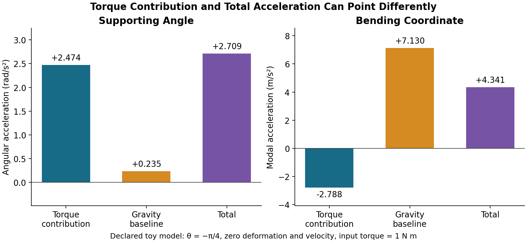
The panels have different physical units and scales. Their bars are components of an instantaneous model calculation, not percentages of swing outcome or experimental estimates of muscle action.
The coordinate sign is a convention: set \(\xi=-\eta\) and simultaneously use shape \(-\phi\). Physical displacement is unchanged, while the cross mass and coupling change sign. A positive coefficient in the transformed coordinates is equally consistent with the same physical response.
Even the frequency depends on the specified boundary experiment. For the linearized zero-gravity model at zero deflection, holding \(\theta\) fixed gives \(f=\sqrt{k/A}/(2\pi)=16.8894\) Hz. Allowing the supporting angle to move freely gives one zero-frequency mode and a nonzero frequency \(\sqrt{k/(A-B^2/J_0)}/(2\pi)=22.0067\) Hz. Neither number establishes a typical shaft frequency, and gravity or a controlled support changes the linearization.
The executable checks independently integrate the distributed kinetic energy, differentiate the potential, verify the power balance and its time integral, solve the input and total accelerations, and check sign transformations and both frequency problems.
Spatial Rigid and Flexible Models
A rigid spatial pendulum with orientation \(R\in SO(3)\), body angular velocity \(\omega\), center vector \(r_C\), and positive-definite pivot inertia \(I\) satisfies
\[ \begin{aligned} \dot R&=R\widehat\omega,\\ I\dot\omega+\omega\times(I\omega)&=u+\tau_g(R),\\ \tau_g(R)&=r_C\times R^\top(0,0,-mg)^\top. \end{aligned} \]
All torques here are body-frame components. The potential is \(U_g=mg\,e_3^\top Rr_C\), and its directional derivative gives the opposite of gravitational virtual work. The gyroscopic term does no work because \(\omega\cdot[\omega\times(I\omega)]=0\). The point-mass/massless-rod limit has singular pivot inertia along the rod; it does not permit this \(I^{-1}\) formulation on all three angular components. A finite rigid body with the stated inertia does.
For a flexible spatial model, let \(T(\eta,\omega,\dot\eta)\) be assembled from the actual body-frame placements, and \(U(R,\eta)\) include gravity and elasticity. Body angular velocity is a velocity variable, not the time derivative of three globally valid orientation coordinates. With \(p_\omega=\partial_\omega T\) and \(p_\eta=\partial_{\dot\eta}T\), the body-rotation and shape balances take the form
\[ \begin{aligned} \dot p_\omega+\omega\times p_\omega&=u+\tau_U-d_\omega,\\ \dot p_\eta-\partial_\eta T+\partial_\eta U&=-d_\eta. \end{aligned} \]
Here \(\tau_U\) is defined by \(\delta U=-\tau_U\cdot\delta\alpha\) for a body rotation \(\delta R=R\widehat{\delta\alpha}\). The inertia is the Hessian of \(T\) in \((\omega,\dot\eta)\).
The rotational variation obeys \(\delta\omega=\delta\dot\alpha+\omega\times\delta\alpha\) rather than the variation of an ordinary coordinate derivative. Holm, Marsden, and Ratiu, equations (1.13)–(1.26), derive this constrained variation and its momentum cross term. Adding free shape-coordinate variations and the declared potential/load terms gives the two balances above.
With positive-definite inertia, these equations can be collected as
\[ \widetilde M(R,\eta) \begin{bmatrix}\dot\omega\\\ddot\eta\end{bmatrix} +\widetilde h(R,\eta,\omega,\dot\eta) =\begin{bmatrix}u\\0\end{bmatrix}. \tag{13}\]
The bias includes the rotational momentum term and all modal potential derivatives. Together with \(\dot R=R\widehat\omega\), it is affine in the declared body torque. Do not apply the ordinary coordinate Christoffel formula to body angular velocity without the additional rotation kinematics. These are structural equations, not a solved three-dimensional golfer simulation.
Verification and Golf Interpretation
These examples connect force transmission, shaft deformation, gravity, coordinate conventions, and energy. They show why an instantaneous torque effect, total acceleration, modal frequency, and delivered contact are different quantities. A passive mode can still accelerate under gravity and inertial coupling; changing the chosen mode coordinate cannot change physical motion; and changing support conditions can change vibration frequencies even with the same material parameters.
Compare independent assemblies, force-balance residuals, energy/work residuals, coordinate transformations, timestep refinement, and mode convergence before interpreting a simulation. Then compare the specified outputs with suitable measurements under declared uncertainty. Such numerical verification does not establish empirical validity. A zero-input forward trajectory is a new initial-value problem, not generally a subtraction of two completed paths. Instantaneous zero-velocity evaluation also retains the declared configuration, parameters, and auxiliary states.
The numerical consistency article describes a reproducible evaluation procedure. No particular Simulink implementation, measured accuracy, optimal golf technique, or biological causal attribution is established by the algebra in this appendix. The primary sources support the engineering methods; the examples and limitations here state what has actually been calculated.
Revision History
2026-09-08: Standardized cross-article category metadata and link targets (#4302).
2026-09-05: Derived loaded beam and reproducible pendulum models with explicit limits (#4193, #4153).
2026-08-29: Governed claim and critique adjudication framework (#4051).
2026-03-10: Three-pass professional assessment and formalization.
Citation
@online{olson,
  author = {Olson, Dieter},
  title = {Theory {Series,} {Part} 4: {Worked} {Pendulum} {Dynamics}},
  date = {},
  url = {https://affinedrift.com/articles/theory-part4.html},
  langid = {en},
  abstract = {This article develops explicit analytical derivations and
    reproducible numerical examples for loaded beam and multi-link
    pendulum models of the golf swing. It explores how shaft
    flexibility, boundary conditions, and actuator torques interact to
    produce non-collinear acceleration components.}
}