Passive Distributed Control: Mechanics and the Bosch Framework
Plain-Language Summary
Body and club parts shape what a golfer can guide. This article links stored spring energy, sensory loops, and balance in a clear model. It keeps those math results separate from unproven claims about skill.
Key Takeaways
- Elastic structures can store and return energy; their loading source, losses and boundary work must still be counted.
- Recurring movement patterns do not alone establish a limit cycle, contraction or a zero-input golf swing.
- The series-spring example has a consistent massless junction and energy balance; its parameters are illustrative rather than identified human measurements.
The Question Behind Passive Distributed Control
The original publication date is unverified; the revision date appears above.
A golfer does not consciously prescribe every muscle force. Nevertheless, forces must act, elastic structures must be loaded, and the club must reach suitable impact conditions. A useful account explains how mechanical structure, retained body states and control signals jointly shape that outcome.
Frans Bosch’s Strength Training and Coordination (2015) motivates an integrated view of coordination and physical preparation. The publisher’s introduction also acknowledges the use of hypothetical models. We use that framework to pose mechanical questions. The equations below are explicit models for examining those questions, not a verbatim Bosch quotation or a derivation of his complete framework.
This article develops the distinctions needed to interpret passive and distributed control. The Physics of Golf, Chapter 27 provides the separate textbook treatment of impedance, pre-tuning and feedback. A result established for one model or chapter does not automatically validate a different example.
Input, Passivity and Feedback Answer Different Questions
A control-affine model has the form
\[ \dot x=f_p(x)+G_p(x)u. \]
Here \(x\) is the complete retained state, \(u\) is the declared input, and \(p\) contains fixed model settings. A torque command, neural excitation and an impedance setting are different input choices. Setting one of them to zero may leave activation, elastic preload, damping and compatible constraint reactions in the model. The zero-torque counterfactual family therefore requires an explicit intervention and construction.
Mechanical passivity instead concerns energy and a boundary power port. For storage \(E\geq0\) and a collocated applied force \(F\) and velocity \(v\), a passive mechanical subsystem satisfies
\[ E(t)-E(0)\leq\int_0^t F(s)v(s)\,ds. \]
A spring can deliver positive power temporarily by releasing initial storage. Its energy came from prior loading or another accounted source. Zero present input does not make that initial energy free. Conversely, a nonzero holding force can have zero mechanical power when its application point is stationary; this says nothing by itself about metabolic expenditure.
The drift \(f_p\) is a state derivative, not a power or an energy source. For a smooth, time-independent storage function,
\[ \dot E=\nabla E(x)^{\mathsf T}f_p(x) +\nabla E(x)^{\mathsf T}G_p(x)u. \]
Those terms need a physical boundary interpretation before they can be called actuator work, dissipation or intersegment transfer. A norm of \(f_p\), or the drift-control capacity ratio, does not establish an energy fraction or muscle-effort fraction.
Feedback adds another distinction. If \(u=\pi(x)\), the resulting autonomous closed-loop field is \(f_p+G_p\pi\). Attraction observed under that policy belongs to the controlled system. Expertise may involve different timing, sensing, impedance or admissible inputs; there is no general theorem that expert performance requires \(u\to0\).
Recurrence, Attraction and the Phase of a Movement
A repeated coordination pattern is an observation. Calling it an attractor requires a stated dynamical system, an invariant set and convergence from nearby initial conditions. Calling it a limit cycle further requires a periodic orbit. A single finite downswing is not itself evidence for an asymptotically stable cycle.
The distinction between ordinary contraction and orbital stability is visible in a simple abstract example. On an annulus containing \(r=1\), with phase \(\theta\) taken modulo \(2\pi\), let
\[ \dot r=-\kappa(r-1),\qquad \dot\theta=\omega, \qquad \kappa>0,\quad\omega>0. \]
Radial errors decay as \(e^{-\kappa t}\), while two trajectories retain their initial phase offset. The circle \(r=1\) attracts transversely. On the section \(\theta=0\), the return time is \(T=2\pi/\omega\) and the transverse return multiplier is \(e^{-\kappa T}<1\). The phase direction of the periodic flow is neutral, with multiplier one. Equal-time convergence of every state direction would be a stronger and different claim.
Manchester and Slotine’s transverse-contraction treatment formalizes orbital convergence under specified dynamical and metric conditions. A coaching label or recurring video pattern does not establish those conditions. For a golf swing, a more direct question is how a declared perturbation changes a later event, such as club delivery, under a specified feedback policy and contact mode.
Practice Variation and Mechanical Impedance
Freezing, freeing and exploiting degrees of freedom are useful descriptions when they have operational meanings. Anatomical configuration dimension, observed movement variability, muscle co-contraction, mechanical impedance and neural feedback gain are separate quantities. Reduced movement at a joint does not show which of these changed.
For a linear mechanical coordinate, let \(m\ddot x+b\dot x+kx=F\) and choose a constant reference \(r\). Instantaneous proportional-derivative feedback with the balancing force is \(F=kr-k_p(x-r)-k_d\dot x\). Then \(e=x-r\) satisfies
\[ m\ddot e+(b+k_d)\dot e+(k+k_p)e=0. \]
Even at zero error and speed, the holding force \(kr\) remains when the reference is nonzero. With \(m>0\), \(k+k_p>0\) and \(b+k_d>0\), this ideal error model is asymptotically stable. Stiffness-like gain changes the undamped natural frequency \(\sqrt{(k+k_p)/m}\), while damping-like gain changes decay and overshoot. This does not make gain identical to bandwidth or uncertainty. Delays, actuator limits, noise and unmodeled modes can alter stability; a better forward prediction does not automatically imply lower feedback bandwidth.
Differential learning uses deliberately varied practice, but universal superiority and a unique neural explanation require evidence. In a 2012 football pilot by Schöllhorn, Hegen and Davids, 24 participants entered and only 12 completed the protocol, four per group. Practice variation and corrective-feedback conditions differed together. Those methodological features limit component-specific causal attribution and transfer to golf; this article does not claim a complete statistical review of that study.
A noise analogy also needs an actual stochastic model. For the illustrative scalar process \(d\xi=-a\xi\,dt+\sigma\,dW_t\), with \(a>0\) and initial variance \(V_0\),
\[ \operatorname{Var}\xi(t)=e^{-2at}V_0+ \frac{\sigma^2}{2a}\left(1-e^{-2at}\right). \]
The variance follows \(\dot V=-2aV+\sigma^2\). Its limiting value depends on both restoring dynamics and forcing; it supplies no universal minimum exploration radius. In several dimensions, unforced directions can remain deterministic. Practice variability, outcome accuracy and learning retention must be measured and compared, rather than inferred from this analogy.
What Passive Walkers Establish
McGeer’s passive-dynamic walking study shows that particular mechanisms can sustain stable stepping down a slope under suitable conditions. Gravitational potential supplies the losses. Existence and stability are separate questions: a periodic stepping solution need not be stable. A return-map calculation must specify the section, impact/reset rule, leg relabeling and reduced state. Absolute downhill position and gravitational potential do not return to their original values each step.
Collins and colleagues’ level-ground robots combine favorable mechanics with actuation and different control architectures. Their results support studying mechanical design together with control. They do not establish that human walking or a golf downswing is an uncontrolled attractor. Mechanical actuator work, electrical consumption and human metabolic cost also have different accounting boundaries.
Tendon Loading Is Not a Muscle-Contraction Label
Tendon extension and muscle-fascicle extension are different measurements. In Fukunaga and colleagues’ walking experiment, six men walked at 3 km/h while ultrasound, EMG, joint motion and ground reaction were recorded. The reported near-isometric fascicle behavior coexisted with estimated tendon stretching during support and recoil during push-off. Thus tendon loading need not require eccentric fascicle motion. This walking evidence does not quantify wrist-tendon behavior in golfers.
Ker and colleagues’ 1987 abstract identifies the foot arch as an elastic contributor during running. That abstract does not verify a particular Achilles percentage or a golf energy budget. We therefore assign no universal percentage here. Any fraction needs its tissue, activity, integration interval, denominator and measurement uncertainty stated.
A load–hold–release sequence can be a modeling choice. It is not a universal optimal strategy demonstrated by the existence of elastic tissue. Tendon hysteresis, slack, force–length–velocity effects, changing geometry and active state evolution matter when replacing an ideal spring with an identified muscle–tendon model.
A Consistent Series-Spring Example
Consider one manufactured horizontal mechanical topology, with no gravitational force along the modeled axis. A mass at displacement \(x\) is connected to fixed ground through two springs, with a massless junction at \(y\). The proximal spring has stiffness \(k_m\) and extension \(x-y\); the distal spring has stiffness \(k_t\) and extension \(y\). A damper \(b\) connects the mass directly to ground. Applied force \(F\) acts at that mass. Displacements are measured from unloaded equilibrium, and both springs are ideal bilateral linear elements. These labels are analogues, not identified muscle or tendon states.
The mass and junction balances are
\[ m\ddot x+b\dot x+k_m(x-y)=F, \qquad k_m(x-y)=k_t y. \]
There is no independent junction velocity law. Solving its algebraic balance and substituting into the mass equation gives
\[ y=\frac{k_m}{k_m+k_t}x,\qquad k_{\rm eff}=\frac{k_mk_t}{k_m+k_t},\qquad m\ddot x+b\dot x+k_{\rm eff}x=F. \]
A relaxation law proportional to the spring-force mismatch would instead add a junction damping mechanism. It would require its own constitutive parameter and dissipation term; a small numerical denominator does not enforce the massless-junction constraint.
With \(v=\dot x\), the reduced state equation is
\[ \frac{d}{dt}\begin{pmatrix}x\\v\end{pmatrix} = \begin{pmatrix}v\\-(bv+k_{\rm eff}x)/m\end{pmatrix} + \begin{pmatrix}0\\1/m\end{pmatrix}F. \]
This is affine in the applied force at fixed parameters. Its storage is
\[ E=\frac12mv^2+\frac12k_m(x-y)^2+\frac12k_t y^2 =\frac12mv^2+\frac12k_{\rm eff}x^2. \]
Multiplying the reduced mass balance by \(v\) yields the power and work identities
\[ \dot E=Fv-bv^2,\qquad E(t)-E(0)=W(t)-D(t), \]
where \(W=\int Fv\,dt\) is signed actuator work and \(D=\int bv^2\,dt\geq0\) is dissipated energy. After \(F\) becomes zero, stored elastic energy can become kinetic energy while total storage decreases. This is a passive mechanical statement with an explicit boundary and preload.
Parameters, Preload and the Force Schedule
| Quantity | Illustrative Value | Unit |
|---|---|---|
| Effective mass \(m\) | 0.45 | kg |
| Grounded damping \(b\) | 50 | N s/m |
| Proximal spring \(k_m\) | 1000 | N/m |
| Distal spring \(k_t\) | 5000 | N/m |
| Initial displacement \(x(0)\) | 0.02 | m |
| Initial speed \(v(0)\) | 0 | m/s |
These values give \(k_{\rm eff}=2500/3\) N/m, \(y(0)=1/300\) m, equal initial spring forces \(50/3\) N, and \(E(0)=1/6\) J. Choosing \(y(0)=0.01\) m independently would instead give spring forces of 10 and 50 N, violating junction balance.
The damping ratio is
\[ \zeta=\frac{b}{2\sqrt{mk_{\rm eff}}}=\sqrt{5/3}>1. \]
The unforced reduced model is overdamped, not an oscillatory catapult. Its parameters have not been fitted to a golfer. We apply 100 N for 0.20 s, 80 N for 0.05 s, then zero for 0.25 s. Changing the applied force to 80 N does not impose an isometric hold; displacement and speed remain dynamical outcomes.
Reproducible Energy Accounting
The reusable solver integrates each constant-force interval separately, carries position, velocity, work and dissipation continuously across switches, and computes \(y\) from the algebraic constraint. The source tests compare sampled motion with an independent matrix-exponential solution. Work, storage and losses are checked together; an energy plot alone would not establish closure. The article source contains the runnable example below. The figure can be enlarged for inspection; its generator uses the same solver without executing Python during site publication.
from src.affine_control.series_elastic_demo import (
    LoadStage, SeriesElasticParameters, simulate_series_elastic,
)
parameters = SeriesElasticParameters()
stages = (LoadStage(0.20, 100.0), LoadStage(0.05, 80.0), LoadStage(0.25, 0.0))
trace = simulate_series_elastic(parameters, stages, initial=(0.02, 0.0))
Regenerate the figure from the repository root:
python -m scripts.build_passive_control_figure articles/figures/passive-control-energy.svg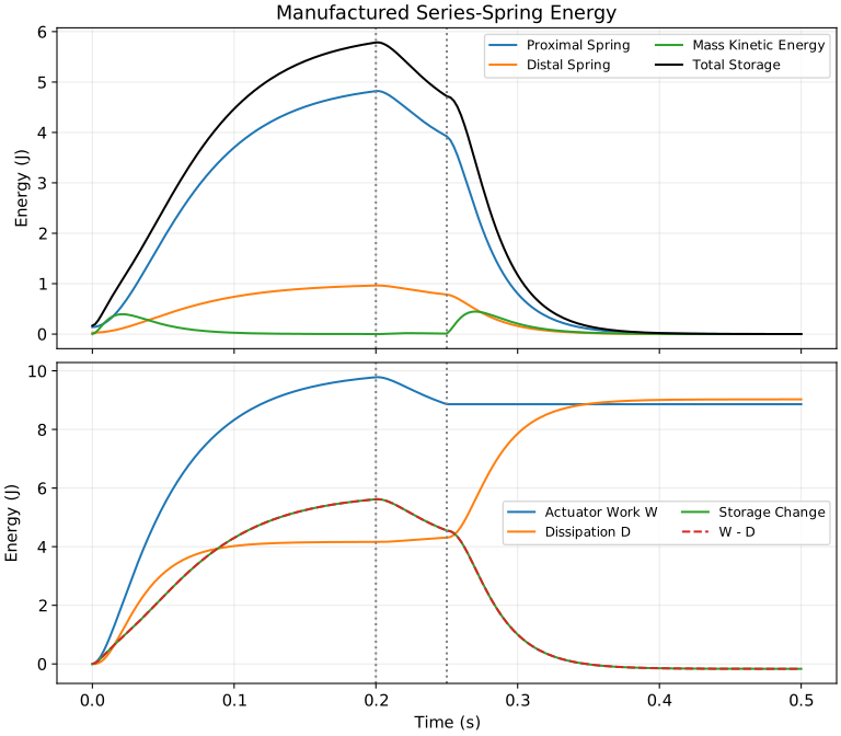
Elastic and kinetic storage appear above; signed actuator work, dissipation and storage change appear below. Dotted lines mark force changes at 0.20 and 0.25 s. The parameters and load schedule are illustrative, with no golfer-specific or muscle-activation inference.
Long Description of the Energy Figure
Both panels use time from zero to 0.5 seconds horizontally and energy in joules vertically. The upper panel separates proximal spring storage, distal spring storage and mass kinetic energy, with their total shown in black. The proximal spring holds the largest share of storage; the initial preload is nonzero. Storage rises during loading and falls toward zero after release.
The lower panel compares accumulated signed actuator work, accumulated damping loss and storage change from the initial state. The dashed work-minus-loss curve overlays the storage-change curve. Work can fall when the mass moves against the applied force, while damping loss continues to rise. After the force becomes zero at 0.25 seconds, actuator work stays constant and the remaining storage is dissipated. Dotted vertical lines mark both force changes.
Actuator work can decrease when force and velocity have opposite signs: the actuator then absorbs mechanical energy. Dissipation can exceed net supplied work by drawing down the initial preload. Both effects are consistent with \(E-E(0)=W-D\); neither is evidence of energy generation.
Coupling and Changing the Plant
In a multibody model, coupling may enter inertia, geometry, constraints and constitutive forces. Even with a diagonal generalized-input map \(B\), solving \(M\ddot q+h=Bu\) can produce a non-diagonal acceleration map \(M^{-1}B\). Constraint-compatible dynamics require the corresponding constrained solve. Off-diagonal entries of a particular \(G\) therefore do not identify fascial transmission or its magnitude.
A proposed connective-tissue pathway needs a constitutive and geometric model, measurements and an uncertainty analysis. Elastic effects cannot be assigned to an inertial or damping matrix merely to call their treatment conservative. The force and mobility reference develops the load-to-acceleration distinction.
Changing impedance also changes the accounting problem. For a hypothetical spring with prescribed positive \(k(t)\), differentiating \(E_s=k(t)x^2/2\) adds the term \(\dot k x^2/2\). A tuning mechanism or expanded internal-state model must account for that energy exchange. The constant-parameter simulation above makes no such intervention. A cue to relax may change several loads, settings and states; it cannot be translated into one universal reduction of input or feedback gain.
A Testable Golf-Swing Interpretation
The useful proposal is that a task can benefit from the interaction of mechanical structure, initial state and control. To make that proposal testable, declare the following together:
- Task and boundary: Which club-delivery outcome is evaluated, over what interval, and which bodies and power ports enter the energy budget?
- Plant and input: Which activation, elastic and controller states remain, which settings are fixed, and what input is varied or set to zero?
- Perturbation and comparison: Which matched initial conditions, feedback policies, constraints and uncertainty model define the counterfactual?
- Measurements and falsifiers: Which predictions would distinguish the proposed mechanism from alternative load sharing or control policies?
EMG and kinematics can constrain parts of this account. They do not alone identify every tendon force, intrinsic impedance, energy transfer or causal control law. Intersegment power accounting and prediction with action selection provide complementary pieces: mechanics determines what a command can do, state determines the immediate response, and the task determines whether that response is useful.
Revision History
2026-10-03: Corrected attribution, stability and learning claims; reconciled the series-spring equations and simulation with explicit energy accounting (#4836).
2026-09-10: Wired motor-control and neuroscience cluster cross-links (#4365).
2026-09-08: Standardized cross-article category metadata and link targets (#4302).
2026-08-13: Fixed definitional integrity and drift-control attribution (#3845).
2026-03-10: Initial publication on passive distributed control integration.
Citation
@online{olson,
  author = {Olson, Dieter},
  title = {Passive {Distributed} {Control:} {Mechanics} and the {Bosch}
    {Framework}},
  url = {https://affinedrift.com/articles/passive-distributed-control.html},
  langid = {en},
  abstract = {A critical translation of passive and distributed control
    into explicit mechanical and dynamical models. The article
    distinguishes input choice, mechanical passivity, orbital stability,
    practice variability and biological inference. A manufactured
    series-spring model enforces junction balance and tracks actuator
    work, storage and dissipation across force changes.}
}